1. Isolated word recognition with the Liquid State Machine: a case study
D. Verstraeten ∗, B. Schrauwen, D. Stroobandt, J. Van Campenhout
Written By:
Gassan Tabajah
Ron Adar
Gil Rapaport

2. Abstract
The Liquid State Machine (LSM) is a recently developed computational model with interesting properties.
It can be used for pattern classification, function approximation and other complex tasks.
Contrary to most common computational models, the LSM does not require information to be stored in some stable state of the system:
The inherent dynamics of the system are used by a memoryless readout function to compute the output.

3. Abstract
In this paper we present a case study of the performance of the Liquid State Machine based on a recurrent spiking neural network by applying it to a well known and well studied problem:
Speech recognition of isolated digits.
We evaluate different ways of coding the speech into spike trains.
In its optimal configuration, the performance of the LSM approximates that of a state-of-the-art recognition system.
Another interesting conclusion is the fact that the biologically most realistic encoding performs far better than more conventional methods.

4. 1. Introduction
Many complex computational problems have a strong temporal aspect:
Not only the value of the inputs is important, but also their specific sequence and precise occurrence in time.
Tasks such as speech recognition, object tracking, robot control or biometrics are inherently temporal, as are many of the tasks that are usually viewed as ‘requiring intelligence’.

5. 1. Introduction
However, most computational models do not explicitly take the temporal aspect of the input into account or transform the time-dependent inputs to static input using.
e.g., a tapped delay line.
These methods disregard the temporal information contained in the inputs in two ways:
The time-dependence of the inputs within a certain time window is compressed into a static snapshot and is therefore partially lost.
The temporal correlation between different windows is not preserved.

6. Liquid State Machine (LSM)
The Liquid State Machine (LSM) avoids these problems by construction.
The LSM is a computational concept (its structure is depicted in Fig. 1):

7. Liquid State Machine (LSM)
A reservoir of recurrently interacting nodes is stimulated by the input u(t),
A running or liquid state x(t) is extracted and a readout function fM converts the high-dimensional liquid state x(t) into the desired output y(t) for the given task.

8. Liquid State Machine (LSM)
The loops and loops within-loops which occur in the recurrent connections between the nodes in the reservoir cause a short-term memory effect to occur:
The influence of inputs fed into the network ‘resonate’ for a while before dying out.
Hence the name liquid: ripples in a pond also show the influence of past inputs.
This property is called temporal integration.

9. Types of liquids
The reservoir or liquid can be any type of network that has sufficient internal dynamics.
Currently several types of liquids have been used:
The echo state machine using a recurrent analog neural network.
A real liquid (water) in a bucket.
A delayed threshold logic network.
A Spiking Neural Network (SNN).
The type of liquid we will be using in this article.

10. Readout function
The actual identity of the readout function is also not explicitly specified;
Indeed, it can be any method of statistical analysis or pattern recognition.
Possible readout functions include linear projection, Fisher discriminant, a perceptron, a feed forward MLP trained with backpropagation or even a Support Vector Machine.
Note that the liquid itself is not trained, but chosen a priori:
A heuristic is used to construct ‘interesting’ liquids in a random manner.
Only the readout function is adapted so that the LSM performs the required task.

11. Separation between the liquid and its readout
The separation between the liquid and its readout function offers two considerable advantages over traditional Recurrent Neural Networks (RNN).
First, the readout function is generally far easier to train than the liquid itself, which is a recurrently connected network.
Furthermore, the structure of the LSM permits several different readout functions to be used with the same liquid, which can each be trained to perform different tasks on the same inputs—and the same liquid.
This means that the liquid only needs to be computed once, which gives the LSM an inherent parallel processing capability without requiring much additional processing power.

12. Similarity between LSM and SVM
The LSM is a computational model that bears strong resemblance to another well-known paradigm:
That of the kernel methods and the Support Vector Machine (SVM).
Here, inputs are classified by first using a non-linear kernel function to project the inputs into a very high-dimensional (often even infinitely dimensional) feature space, where the separation between the classes is easier to compute (and can often even be linearly separable).
The LSM can be viewed as a variation:
Here too, the inputs are non-linearly projected into a high-dimensional space (the space of the liquid state) before the readout function computes the output.
The main difference is the fact that the LSM—contrary to SVMs—has an inherent temporal nature.

13. Similarity between LSM and RNN
Another similarity can be found in a the state-of-the-art RNN training algorithm called Backpropagation Decorrelation presented in [6], which was derived mathematically.
It has been shown that training a RNN with this algorithm implicitly also keeps a pool of connections almost constant and only trains the connections to the output nodes.
This behavior is very similar to the principle of the LSM, specifically when using a perceptron as readout function.

14. Filter approximation
In [7] it has been shown that any time invariant filter with fading memory can be approximated with arbitrary precision by a LSM, under very unrestrictive conditions.
In practice, every filter that is relevant from a biological or engineering point of view can be approximated.

15. Article structure This article is structured as follows:
In Section 2 we first detail the setup used to perform the experiments.
In Section 3 we briefly introduce and subsequently test three different speech front ends which are used to transform the speech into spike trains.
The effects of different types of noise that are commonly found in real world applications are tested in Section 4.
In Section 5 we make some relevant comparisons with related isolated word recognition systems.
In Section 6 we draw some conclusions about the speech recognition capabilities of this computational model.
In Section 7 we point out some possible opportunities for further research.

16. Experimental Setup Matlab LSM toolbox Liquid is a
recurrent network (contains loops)
of leaky integrate and fire neurons
arranged in a 3D column (pile)
Parameters taken from original LSM paper

17. Network structure Connections between neurons allocated stochastically
D = Euclidean distance between neurons a, b
C = 0.3/EE, 0.2/EI, 0.4/IE, 0.1/II
Lambda = 2
Effectively: mainly local, limited global connectivity

18. Dataset – subset of TI46
46-word speaker dependant isolated word speech database
500 samples
5 different speakers
Digits ‘zero’ through ‘nine’
10 different utterances
300 training, 200 test

19. Readout function Simple linear projection Winner take all selection
y = output
x = liquid state
w = weight matrix
Winner take all selection
Maximal y value taken as result
Recompute every 20ms, take maximum again

20. Performance metric WER – Word Error Rate
Fraction of incorrectly classified words as a percentage of total number of words

21. Transforming signals to spikes
Voice is an analog signal
Usually even after it is being preprocessed
SNN liquid needs spike trains
BSA: a heuristic algorithm for deciding at each timestamp whether a spike should be emitted

22. Preprocessing Common practice in speech recognition
Enhances speech specific features
Used algorithms
Hopfield-Brody
MFCC
Lyon Passice Ear

23. Hopfield-Brody FFT the sound Examine 20 specific frequencies
Look for onset, offset, peak events
Constantly monitor the same 40 events
Each one is considered a spike train
Treat event time as spike
No need for BSA

24. Hopefield-Brody (cont’)
Not suitable at all
WER first drops when network size increases, but then increases again
Even the best liquids identified 1 in 5 words correctly

25. Mel Frequency Cepstral Coefficients
De-facto standard for speech preprocessing
Hamming Windowing
FFT the signal
Mel-scale filter the magnitude
Log10 the values
Cosine transform – reduce dimensionality, enhance speech features

26. Hamming windowing

27. Mel Scale

28. MFCC (cont’)
Result is the so-called ‘cepstrum’: 13 coefficients of processed analog signal
Compute first and second time-derivatives: total of 39 coefficients
BSA turns them into 39 spike trains fed into LSM
Performance: identifies 1 in 2 words

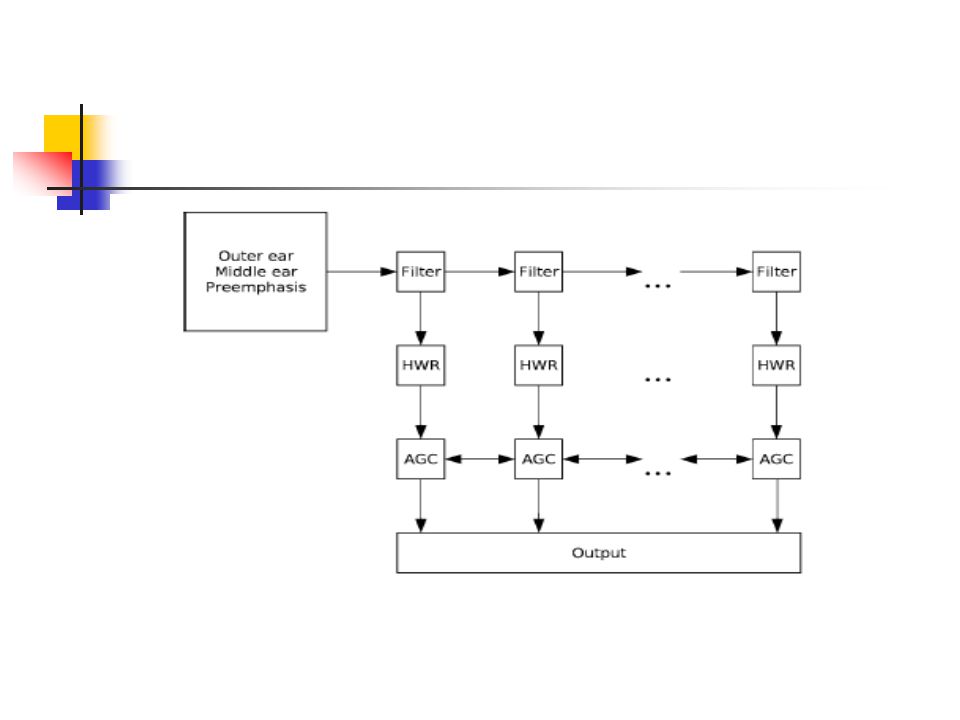
29. Lyon passive ear
A model of human inner ear (cochlea), on the name of Richard F. Lyon.
Describes the way acoustic energy is transformed and converted to neural representations.
Considered to be simple model comparing to others.

30. Lyon passive ear cont’ Model consists of:
1) filter bank-closely resembles the selectivity of the human ear
to certain frequencies.
2) a series of half-wave rectifies (HWRs) and adaptive
gain controllers (AGCs) both of them modeling the hair cells
response.
3) Each filter output, after detection and AGC, is called a
channel.

32. The Peripheral Auditory System
Auditory nerve
Cochlea
Outer Ear
Middle
Ear
Inner
Ear 32

33. Performance
Performance results for LPE(WER=word error rate)

34. Cochleagram
Full time sequence of the outputs of the last stage.

35. The hall process

36. Input with noise
To test the robustness robustness of the recognition performance to noisy environments, a noise is added to the input.
Different types of noise have been used:
1) speech babble
2) white noise
3) interior noise
The LSM was compared to the best results from one of the books in the references, which was the “Log Auditory Model” (LAM) with noise robust front-end.

37. Input with noise cont’
The LAM designed for noise robustness and it followed by Hidden Markov Model (HMM).
Here we can see a table that compares LSM to LAM with different kind of noise, and in levels of 10,20, 30 dB, tested on single liquid with 1232 neurons, trained on clean speech and tested on noisy speech.

38. Comparison to other machines
Sphinx4 is a recent speech recognition system (by Sun Microsystems) using HMMs and MFCC front end. On the database TI46 get error rate of 0.168%, compare to 0.5% on the best LSM from the experiment.
But LSM also have couple of advantages over HMMs:
HMMs tends to be sensitive to noisy inputs.
Usually biased towards a certain speech database.
Do not offer a way to perform additional tasks like speaker identification or word separation on the same input without dramatic increase in computational.

39. Conclusion
The paper have looked the SNN interpretation of the LSM to the task of isolated word recognition with a limited vocabulary.
Several methods of transforming the sounds into spikes train have been explored.
The results showed that LSM is well suited for the task, and that the performance is far better using biological model (LPEM).
LSM also worked well with noise on the input (noise robustness).

40. Future work
Find out what causes the big difference between LPE model to the traditional MFCC methods.
Further research is needed in order to find a hardware implementation to parallel LSM that could keep the dynamics of the current LSM.