Download presentation
Presentation is loading. Please wait.

1
Advances in Earthquake Location and Tomography William Menke Lamont-Doherty Earth Observatory Columbia University

2
Part 1: Advantage of using differential arrival times to locate earthquakes Part 2: Simultaneous earthquake location and tomography Part 3: In depth analysis of the special case of unknown origin time Outline

3
Part 1 Advantage of using differential arrival times to locate earthquakes

5
that was the recent Gulf of Mexico earthquake, by the way …

6
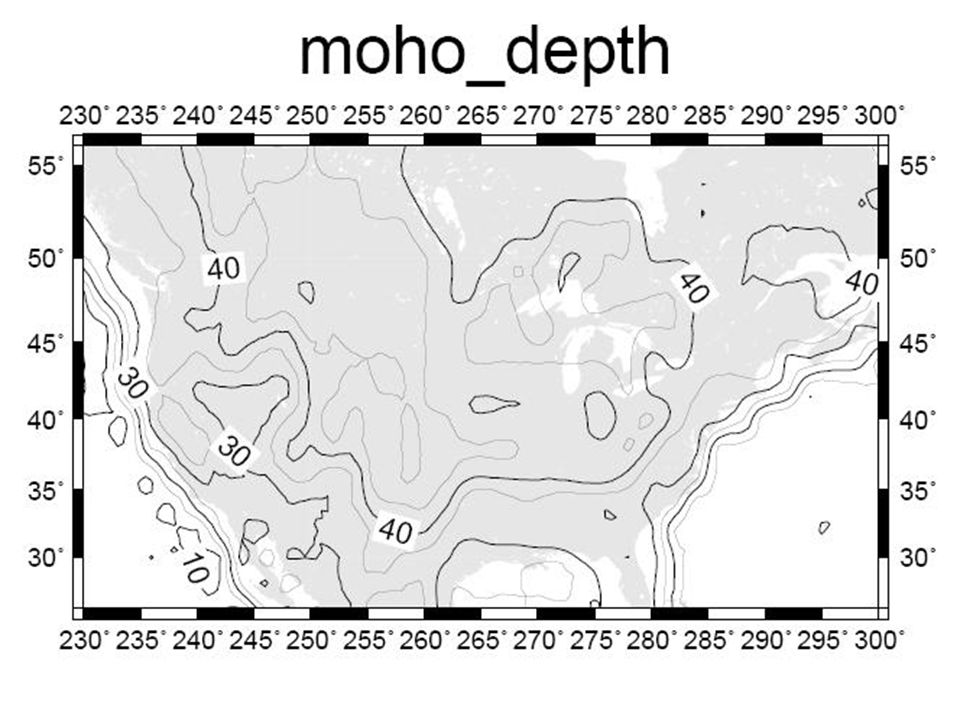
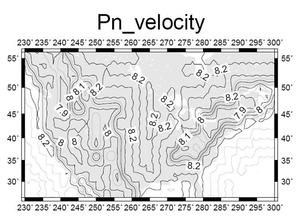
Locating an earthquake requires knowing the seismic velocity structure accurately

10
What’s the best way to represent 3 dimensional structure Best for what? compatibility with data sources ease of visualization and editing facilitating calculation

11
Overall organization into interfaces Small-scale organization into tetrahedra Linear interpolation within tetrahedra implying rays that are circular arcs

12
seismometerearthquake

13
Location Errors: = 0.5 degree = 55 km = 30 miles Note: this preliminary calculation used data from a limited number of stations

14
Two parallel approaches work to improve earth model design earthquake location techniques that are as insensitive to model as possible

15
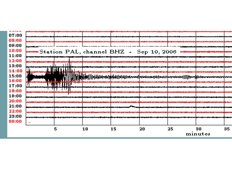
Waves from earthquake first arrived in Palisades NY at 15:00:32 on Sept 10, 2006

17
Arrival Time ≠Travel Time Q: a car arrived in town after traveling for an half an hour at sixty miles an hour. Where did it start? A. Thirty miles away Q: a car arrived in town at half past one, traveling at sixty miles an hour. Where did it start? A. Are you crazy?

18
Suppose you contour arrival time on surface of earth Earthquake’s (x,y) is center of bullseye but what about its depth?
 is center of bullseye but what about its depth")
19
Earthquake’s depth related to curvature of arrival time at origin Deep Shallow

22
Courtesty of Felix Walhhauser, LDEO Earthquakes in Long Valley Caldera, California located with absolute traveltimes

23
Courtesty of Felix Walhhauser, LDEO Earthquakes in Long Valley Caldera, California located with differential traveltimes

24
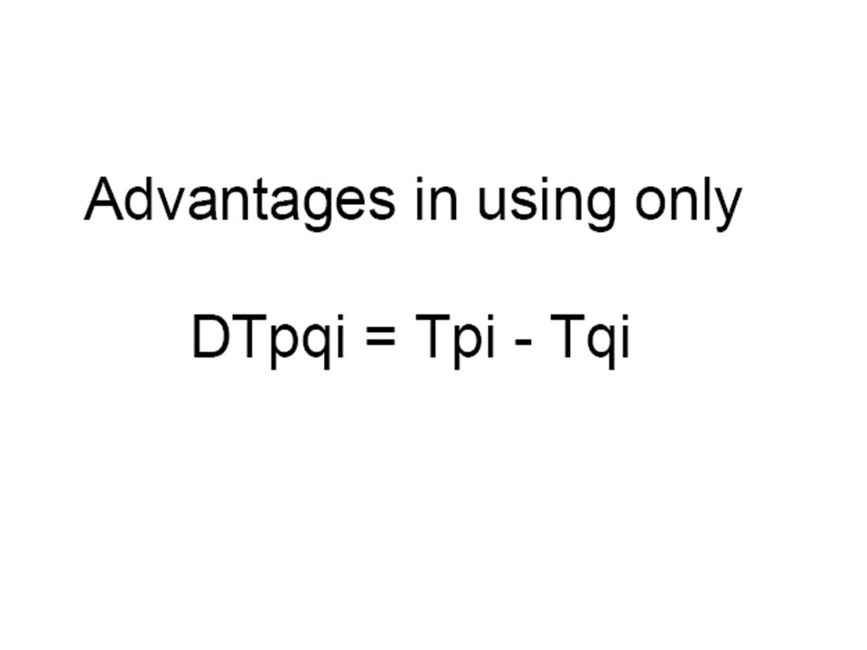
differential arrival time = difference in arrival times

25
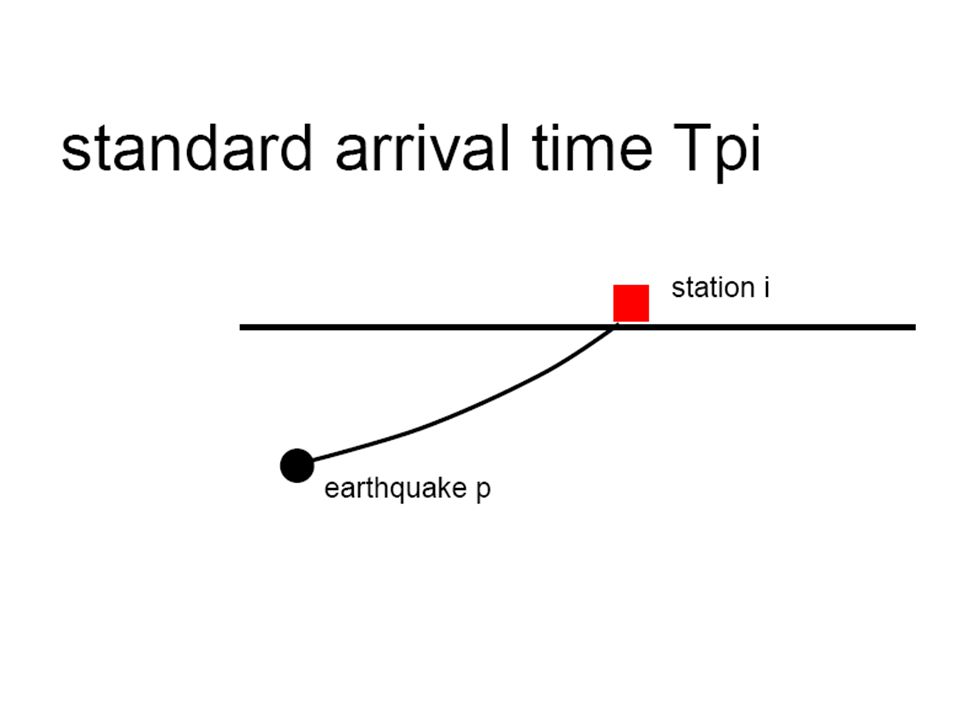
T = arrival time TT = travel time To = Origin Time (start time of earthquake) mean origin time cancels out
 mean origin time cancels out")
26
Station i

28
Very accurate DT’s !

29
A technical question for Applied Math types … Are differential arrival times as calculated by cross-correlation less correlated than implied by the formula They seem to be. If so, the this is another advantage of using the method

31
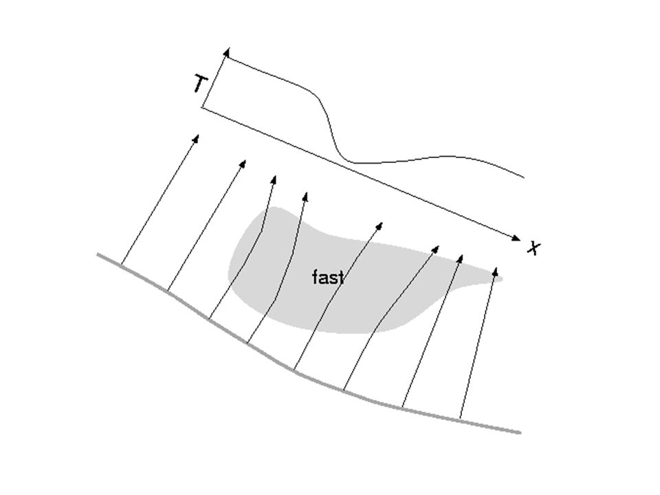
How does differential arrival time vary spatially? Depends strongly on this angle

32
In a 3 dimensional homogeneous box … maximum mean minimum If you can identify the line AB, then you can locate earthquakes

33
as long as you have more than two earthquakes

34
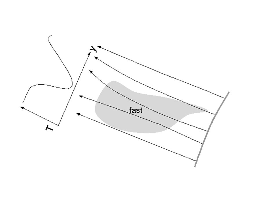
In a vertically-stratified earth, rays are bent back up to the surface, so both Points A and B are on the surface. The pattern of differnetial traveltime is more complicated … ray wavefront

35
The same idea works … p q

36
Patterns of differential arrival time C C C C C B C B B A AA B A Can you guess the orientation of the two sources in these six cases?

37
This pattern an be seen in actual data, in this case from a pair of earthquakes on the San Andreas Fault Boxes: differential arrival times observed at particular stations Shading: theoretical calculation for best- fitting locations of the earthquake pair C A B

38
Another example …

39
What is the practical advantage of using differential arrival times to locate earthquakes My approach is to examine the statistics of location errors using numerical simulations Compare the result of using absolute arrival time data And differential arrival time data When the data are noise Or the earth structure is poorly known

40
Geometry of the numerical experiment …

41
Effect of noisy data (10 milliseconds of measurement error) absolute data differential data
 absolute data differential data")
42
Effect of near surface heterogeneities (1 km/s of velocity variation with a scale length of 5 km) absolute data differential data absolute data
 absolute data differential data absolute data")
43
Both absolute locations and relative locations of earthquakes are improved by using differential arrival time data when arrival times are nosily measured and when near-surface earth structure is poorly modeled Relative location errors can be just a few meters even when errors are “realistically large”

44
Part 2 Simultaneous earthquake location and tomography

48
simultaneous earthquake location and tomography? Many earthquakes with unknown X, Y, Z, To Unknown velocity structure Solve for everything Using either absolute arrival times or differential arrival times

49
A numerical test 11 stations 50 earthquakes on fault zone Heterogeneity near fault zone only

50
True earthquake locations And fault zone heterogenity ( 1 km/s) Reconstructed earthquake locations And fault zone heterogenity, using noise free differential data Note the amplitude of the “signal” is only 1 ms, so noise might be a problem.
 Reconstructed earthquake locations And fault zone heterogenity, using noise free differential data Note the amplitude of the signal is only 1 ms, so noise might be a problem.")
51
Reality Check: How big is the Signal? How much better are the data fit? When the earth structure is allowed to vary compared with holding a simple, layered earth structure fixed? Answer: 0.7 milliseconds, for a dataset that has traveltimes of a few seconds Need very precise measurements!

52
Part 3 Is Joint Tomography/Earthquake Location Really Possible ? Study a simplified version of the problem In depth analysis of the special case of unknown origin time but known location

55
Station 1 2 3 4 Event 1 Event 2 Event 3

56
If you can … Then that structure is indistinguishable from a perturbation in origin time!

57
Case of sources near bottom of the model This velocity perturbation causes constant travel time perturbation for a station on the surface anywhere in the grey box for the event at but zero traveltime perturbation for all the sources at !

58
Case of sources near top of model This velocity perturbation causes constant travel time perturbation for a station on the surface anywhere in the grey box for the event at but zero traveltime perturbation for all the sources at !

59
But you can always find such structures! And they often look ‘geologically interesting’ Yet their presence of absence in an area cannot be proved or disproved by the tomography.

60
Summary Part 1: Earthquake location with differential data is the way to go! Part 2: Simultaneous tomography / earthquake location possible with differential data, but requires high-precision data. Part 3: Coupled Tomography/Location is extremely nonunique and extremely likely to fool you.

Similar presentations


![Lecture 4: Practical Examples. Remember this? m est = m A + M [ d obs – Gm A ] where M = [G T C d -1 G + C m -1 ] -1 G T C d -1.](/16/5018683/big_thumb.jpg "Lecture 4: Practical Examples. Remember this? m est = m A + M [ d obs – Gm A ] where M = [G T C d -1 G + C m -1 ] -1 G T C d -1.>")


