Download presentation
Presentation is loading. Please wait.

1
New Spectral Classification Technique for Faint X-ray Sources: Quantile Analysis JaeSub Hong Spring, 2006 J. Hong, E. Schlegel & J.E. Grindlay, ApJ 614, 508, 2004 The quantile software (perl and IDL) is available at http://hea-www.harvard.edu/ChaMPlane/quantile.
 is available at")
2
Extracting Spectral Properties or Variations from Faint X-ray sources Hardness Ratio HR 1 =(H-S)/(H+S) or HR 2 = log 10 (H/S) e.g. S: 0.3-2.0 keV, H: 2.0-8.0 keV X-ray colors C 21 = log 10 (C 2 /C 1 ) : soft color C 32 = log 10 (C 3 /C 2 ) : hard color e.g. C 1 : 0.3-0.9 keV, C 2 : 0.9-2.5 keV, C 3 : 2.5-8.0 keV
 : soft color C 32 = log 10 (C 3 /C 2 ) : hard color e.g. C 1 : keV, C 2 : keV, C 3 : keV.")
3
Hardness Ratio Pros Easy to calculate Require relatively low statistics (> 2 counts) Direct relation to Physics (count flux) Cons Different sub-binning among different analysis Many cases result in upper or lower limits Spectral bias built in sub-band selection Pros Easy to calculate Require relatively low statistics (> 2 counts) Direct relation to Physics (count flux) Cons Different sub-binning among different analysis Many cases result in upper or lower limits Spectral bias built in sub-band selection
 Direct relation to Physics (count flux) Cons Different sub-binning among different analysis Many cases result in upper or lower limits Spectral bias built in sub-band selection Pros Easy to calculate Require relatively low statistics (> 2 counts) Direct relation to Physics (count flux) Cons Different sub-binning among different analysis Many cases result in upper or lower limits Spectral bias built in sub-band selection")
4
Hardness Ratio Pros Easy to calculate Require relatively low statistics (> 2 counts) Direct relation to Physics (count flux) Cons Different sub-binning among different analysis Many cases result in upper or lower limits Spectral bias built in sub-band selection Pros Easy to calculate Require relatively low statistics (> 2 counts) Direct relation to Physics (count flux) Cons Different sub-binning among different analysis Many cases result in upper or lower limits Spectral bias built in sub-band selection e.g. simple power law spectra (PLI = ) on an ideal (flat) response S band : H band ~ 0 ~ 1 ~ 2 0.3 – 4.2 : 4.2 – 8.0 keV = 1:1 4:1 27:1 0.3 – 1.5 : 1.5 – 8.0 keV = 1:5 1:15:1 0.3 – 0.6 : 0.6 – 8.0 keV = 1:24 1:41:1
 on an ideal (flat) response S band : H band ~ 0 ~ 1 ~ – 4.2 : 4.2 – 8.0 keV = 1:1 4:1 27:1 0.3 – 1.5 : 1.5 – 8.0 keV = 1:5 1:15:1 0.3 – 0.6 : 0.6 – 8.0 keV = 1:24 1:41:1.")
5
Hardness Ratio Pros Easy to calculate Require relatively low statistics (> 2 counts) Direct relation to Physics (count flux) Cons Many cases result in upper or lower limits Spectral bias built in sub-band selection Pros Easy to calculate Require relatively low statistics (> 2 counts) Direct relation to Physics (count flux) Cons Many cases result in upper or lower limits Spectral bias built in sub-band selection e.g. simple power law spectra (PLI = ) on an ideal (flat) response S band : H bandSensitive to (HR~0) 0.3 – 4.2 : 4.2 – 8.0 keV ~ 0 0.3 – 1.5 : 1.5 – 8.0 keV ~ 1 0.3 – 0.6 : 0.6 – 8.0 keV ~ 2
 on an ideal (flat) response S band : H bandSensitive to (HR~0) 0.3 – 4.2 : 4.2 – 8.0 keV ~ – 1.5 : 1.5 – 8.0 keV ~ – 0.6 : 0.6 – 8.0 keV ~ 2.")
6
X-ray Color-Color Diagram C 21 = log 10 (C 2 /C 1 ) C 32 = log 10 (C 3 /C 2 ) C 1 : 0.3-0.9 keV C 2 : 0.9-2.5 keV C 3 : 2.5-8.0 keV Power-Law : & N H Intrinsically Hard More Absorption
 C 32 = log 10 (C 3 /C 2 ) C 1 : keV C 2 : keV C 3 : keV Power-Law : & N H Intrinsically Hard More Absorption")
7
X-ray Color-Color Diagram Simulate 1000 count sources with spectrum at the grid nods. Show the distribution (68%) of color estimates for each simulation set. Very hard and very soft spectra result in wide distributions of estimates at wrong places.
 of color estimates for each simulation set. Very hard and very soft spectra result in wide distributions of estimates at wrong places..")
8
X-ray Color-Color Diagram Total counts required in the broad band (0.3- 8.0 keV) to have at least one count in each of three sub-energy bands Sensitive to C 21 ~0 and C 32 ~0
 to have at least one count in each of three sub-energy bands Sensitive to C 21 ~0 and C 32 ~0")
9
Use counts in predefined sub-energy bins. Count dependent selection effect Misleading spacing in the diagram Use counts in predefined sub-energy bins. Count dependent selection effect Misleading spacing in the diagram Hardness ratio & X-ray colors

10
Use counts in predefined sub-energy bins. Count dependent selection effect Misleading spacing in the diagram Use counts in predefined sub-energy bins. Count dependent selection effect Misleading spacing in the diagram Hardness ratio & X-ray colors e.g. simple power law spectra (PLI = ) on an ideal (flat) response S band, H bandSensitive to Median 0.3 – 4.2, 4.2 – 8.0 keV ~ 04.2 keV 0.3 – 1.5, 1.5 – 8.0 keV ~ 11.5 keV 0.3 – 0.6, 0.6 – 8.0 keV ~ 20.6 keV
 on an ideal (flat) response S band, H bandSensitive to Median 0.3 – 4.2, 4.2 – 8.0 keV ~ 04.2 keV 0.3 – 1.5, 1.5 – 8.0 keV ~ 11.5 keV 0.3 – 0.6, 0.6 – 8.0 keV ~ 20.6 keV.")
11
Search energies that divide photons into predefined fractions. : median, terciles, quartiles, etc Search energies that divide photons into predefined fractions. : median, terciles, quartiles, etc How about Quantiles? e.g. simple power law spectra (PLI = ) on an ideal (flat) response S band, H bandSensitive to Median 0.3 – 4.2, 4.2 – 8.0 keV ~ 04.2 keV 0.3 – 1.5, 1.5 – 8.0 keV ~ 11.5 keV 0.3 – 0.6, 0.6 – 8.0 keV ~ 20.6 keV
 on an ideal (flat) response S band, H bandSensitive to Median 0.3 – 4.2, 4.2 – 8.0 keV ~ 04.2 keV 0.3 – 1.5, 1.5 – 8.0 keV ~ 11.5 keV 0.3 – 0.6, 0.6 – 8.0 keV ~ 20.6 keV.")
12
Quantiles Quantile Energy (E x% ) and Normalized Quantile (Q x ) x% of total counts at E < E x% Q x = (E x% -E lo ) / (E lo -E up ), 0<Q x <1 e.g. E lo = 0.3 keV, E up =8.0 keV in 0.3 – 8.0 keV Median (m=Q 50 ) Terciles (Q 33, Q 67 ) Quartiles (Q 25, Q 75 )
 Terciles (Q 33, Q 67 ) Quartiles (Q 25, Q 75 ).")
13
Quantiles Low count requirements for quantiles: spectral-independent 2 counts for median 3 counts for terciles and quartiles No energy binning required Take advantage of energy resolution Optimal use of information

14
Hardness Ratio HR 1 = (H-S)/(H+S) -1 < HR 1 < 1 HR 1 = (H-S)/(H+S) -1 < HR 1 < 1 HR 2 = log 10 [ (1+HR 1 )/(1-HR 1 ) ] m=Q 50 = (E 50% -E lo )/(E up -E lo ) 0 < m < 1 m=Q 50 = (E 50% -E lo )/(E up -E lo ) 0 < m < 1 Median HR 2 = log 10 (H/S) - < HR 2 < HR 2 = log 10 (H/S) - < HR 2 < qDx= log 10 [ m/(1-m) ] - < qDx < qDx= log 10 [ m/(1-m) ] - < qDx <
![Hardness Ratio HR 1 = (H-S)/(H+S) -1 < HR 1 < 1 HR 1 = (H-S)/(H+S) -1 < HR 1 < 1 HR 2 = log 10 [ (1+HR 1 )/(1-HR 1 ) ] m=Q 50 = (E 50% -E lo )/(E up -E lo ) 0 < m < 1 m=Q 50 = (E 50% -E lo )/(E up -E lo ) 0 < m < 1 Median HR 2 = log 10 (H/S) - < HR 2 < HR 2 = log 10 (H/S) - < HR 2 < qDx= log 10 [ m/(1-m) ] - < qDx < qDx= log 10 [ m/(1-m) ] - < qDx < ](http://images.slideplayer.com/16/4978140/slides/slide_14.jpg "Hardness Ratio HR 1 = (H-S)/(H+S) -1 < HR 1 < 1 HR 1 = (H-S)/(H+S) -1 < HR 1 < 1 HR 2 = log 10 [ (1+HR 1 )/(1-HR 1 ) ] m=Q 50 = (E 50% -E lo )/(E up -E lo ) 0 < m < 1 m=Q 50 = (E 50% -E lo )/(E up -E lo ) 0 < m < 1 Median HR 2 = log 10 (H/S) - < HR 2 < HR 2 = log 10 (H/S) - < HR 2 < qDx= log 10 [ m/(1-m) ] - < qDx < qDx= log 10 [ m/(1-m) ] - < qDx < ")
15
Hardness ratio simulations (no background) S:0.3-2.0 keV H:2.0-8.0 keV Fractional cases with upper or lower limits
 S: keV H: keV Fractional cases with upper or lower limits")
16
Hardness Ratio vs Median (no background) Hardness Ratio 0.3-2.0-8.0 keV Median 0.3-8.0 keV
 Hardness Ratio keV Median keV")
17
Hardness Ratio vs Median (source:background = 1:1) Hardness Ratio 0.3-2.0-8.0 keV Median 0.3-8.0 keV
 Hardness Ratio keV Median keV")
18
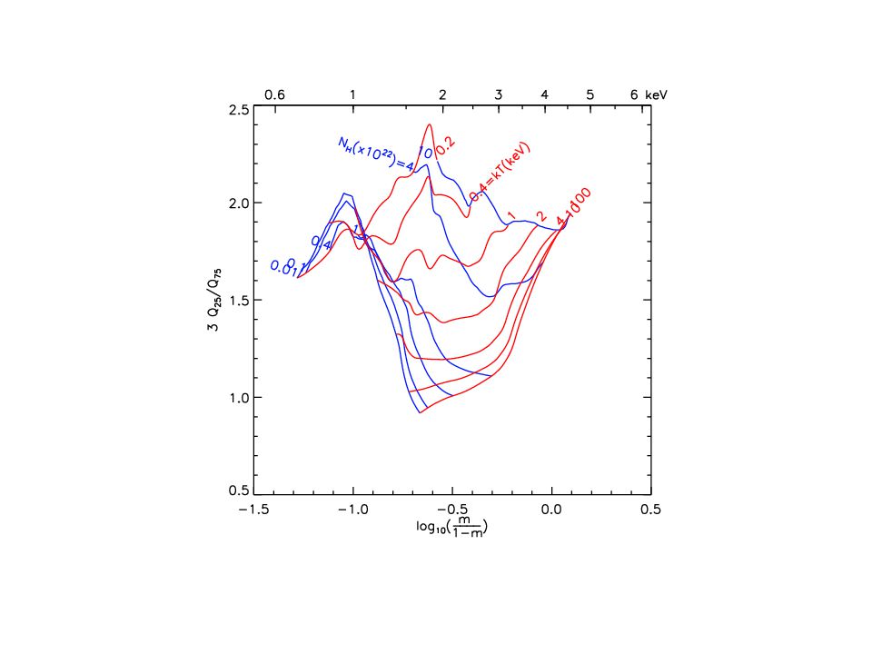
Quantile-based Color-Color Diagram (QCCD) Quantiles are not independent m=Q 50 vs Q 25 /Q 75 Power-Law : & N H Proper spacing in the diagram Poor man’s Kolmogorov -Smirnov (KS) test An ideal detector 03-8.0 keV Intrinsically Hard More Absorption E 50% =
 Quantiles are not independent m=Q 50 vs Q 25 /Q 75 Power-Law : & N H Proper spacing in the diagram Poor man’s Kolmogorov -Smirnov (KS) test An ideal detector keV Intrinsically Hard More Absorption E 50% =")
19
Overview of the QCCD phase space

20
Color estimate distributions (68%) by simulations for 1000 count sources Quantile Diagram 0.3-8.0 keV Conventional Diagram 0.3-0.9-2.5-8.0 keV E 50% =
 by simulations for 1000 count sources Quantile Diagram keV Conventional Diagram keV E 50% =")
21
Realistic simulations ACIS-S effective area & energy resolution An ideal detector E 50% =

22
100 count source with no background Quantile Diagram 0.3-8.0 keV Conventional Diagram 0.3-0.9-2.5-8.0 keV

23
100 source count/ 50 background count Quantile Diagram 0.3-8.0 keV Conventional Diagram 0.3-0.9-2.5-8.0 keV

24
50 count source without background Quantile Diagram 0.3-8.0 keV Conventional Diagram 0.3-0.9-2.5-8.0 keV

25
50 source count/ 25 background count Quantile Diagram 0.3-8.0 keV Conventional Diagram 0.3-0.9-2.5-8.0 keV

26
Energy resolution and Quantile Diagram E lo = 0.3 keV E hi = 8.0 keV E/E = 10% at 1.5 keV E 50% : from E lo + f E lo to E hi – f E hi from ~ 0.4 keV to ~ 7.8 keV

27
Energy resolution and Quantile Diagram E lo = 0.3 keV E hi = 8.0 keV E/E = 20% at 1.5 keV E 50% : from E lo + f E lo to E hi – f E hi from ~ 0.4 keV to ~ 7.6 keV

28
Energy resolution and Quantile Diagram E lo = 0.3 keV E hi = 8.0 keV E/E = 50% at 1.5 keV E 50% : from E lo + f E lo to E hi – f E hi from ~ 0.5 keV to ~ 7.0 keV

29
Energy resolution and Quantile Diagram E lo = 0.3 keV E hi = 8.0 keV E/E = 100% at 1.5 keV E 50% : from E lo + f E lo to E hi – f E hi from ~ 0.7 keV to ~ 6.5 keV

30
Energy resolution and Quantile Diagram E lo = 0.3 keV E hi = 8.0 keV E/E = 200% at 1.5 keV E 50% : from E lo + f E lo to E hi – f E hi from ~ 1.0 keV to ~ 6.0 keV

31
Energy resolution and Quantile Diagram E lo = 0.3 keV E hi = 8.0 keV E/E = 500% at 1.5 keV E 50% : from E lo + f E lo to E hi – f E hi from ~ 1.2 keV to ~ 5.0 keV

32
E/E = 10% at 1.5 keV E/E = 100% at 1.5 keV Energy resolution and Quantile Diagram

33
Sgr A* (750 ks Chandra )
")
34
Sgr A* (750 ks Chandra )
")
35
Sgr A* (750 ks Chandra )
")
36
Sgr A* (750 ks Chandra )
")
37
Sgr A* (750 ks Chandra )
")
39
Swift XRT Observation of GRB Afterglow GRB050421 : Spectral softening with ~ constant N H GRB050509b : Short burst afterglow, softer than the host Quasar

40
Spectral Bias Stability Sub-binning Phase Space Sensitivity Energy Resolution Physics Quantile Analysis None Good No Need Meaningful Evenly Good Sensitive Indirect X-ray Hardness Ratio or Colors Yes Upper/Lower Limits Required Misleading? Selectively Good Insensitive Direct Score Board

41
Future Work Find better phase spaces. Handle background subtraction better. Find better error estimates: half sampling, etc. Implement Bayesian statistics?

43
Conclusion: Quantile Analysis Stable spectral classification with limited statistics No energy binning required Take advantage of energy resolution Quantile-based phase space is a good indicator of spectral sensitivity of the detector. The basic software (perl and IDL) is available at http://hea-www.harvard.edu/ChaMPlane/quantile.
 is available at")
44
In principle, by simulations: slow and redundant Maritz-Jarrett Method : bootstrapping Q 25 & Q 75 : not independent MJ overestimates by ~10% 100 count source: consistent within ~5% Quantile Error Estimates

45
by Maritz-Jarrett Method PL: =2, N H =5x10 21 cm -2 >~30 count : within ~ 10% <~30 count : overestimate up to ~50% MJ requires 3 counts for Q 50 5 counts for Q 33, Q 67 6 counts for Q 25, Q 75 mj / sim

Similar presentations


 Characterization of the soft proton.>")
>")

. HXD: 10-600 keV WAM: 50keV-5MeV XIS: 0.2-12keV X-ray Afterglow (XIS + HXD withToO) Wide energy band (0.2-600 keV) Ultra-low.>")

-CsI(Na) phoswich 0.05–10 4ms COMPTELNaI0.7–300.1s EGRET TASCSNaI(Tl)1-2001s.>")
 & G350.1-0.3 in X-rays Anant Tanna Physics IV 2007 Supervisor: Prof. Bryan Gaensler.>")


 Makoto Tashiro,>")


 ABSTRACT: We present spectral fits for RHESSI and GOES solar.>")


