1. WFM 6202: Remote Sensing and GIS in Water Management
[Part-B: Geographic Information System (GIS)]
Lecture-2: Data Model and Structure
Dr. Akm Saiful Islam
Institute of Water and Flood Management (IWFM)
Bangladesh University of Engineering and Technology (BUET)
November, 2008

2. Data Model
A set of guidelines to convert the real world (called entity) to the digitally and logically represented spatial objects consisting of the attributes and geometry.
Types of geometric data model
Vector Model
Model uses discrete points, lines and areas corresponding to discrete objects with name or code number of attributes
Raster Model
- Model uses regularly spaced grid cells in specific sequence. An element of grid cell is called a pixel (picture cell)

3. Vector and Raster Model
Vector model
more colors
256 color
Raster model

4. Example of vector based model

5. Raster model
Raster model, otherwise known as a raster dataset (image), in its simplest form is a matrix (grid) of cells.
Cell value - Each cell has a value.
Cell size- Each cell has a width and height and is a portion of the entire area represented by the raster
Cell location - The location of each cell is defined by its row or column location within the raster matrix.

6. Example of raster representation

7. Comparison of Raster and Vector Data Model Advantages
Raster model
Vector model
1. It is a simple data structure
1. It provides a more compact data structure that the raster model
2. Overlay operations are easily and efficiently implemented
2. It provides efficiently encoding of topology and as result more efficiently implementation of operation such as network analysis
3. High Spatial variability is efficiently represented in raster format
3. The vector model is better suited to supporting graphics that closely approximate Hand-drawing maps
4. The raster format is more or less required for efficient manipulation and enhancement of digital images

8. Comparison of Raster and Vector Data Model Disadvantages
Raster model
Vector model
1. It is less compact therefore data compression techniques can often overcome this problem.
1. It is a mode complex data structure.
2. Topological relationships are more difficult to represent.
2. Overlay operations are more difficult to implement.
3. The output of graphics is less aesthetically pleasing because boundaries tend to have a blocky appearance rather than the smooth lines of hand-drawn maps.
3. The representation of high spatial variability is inefficient.
4. Manipulation and enhancement of digital images cannot be effectively done in vector domain.

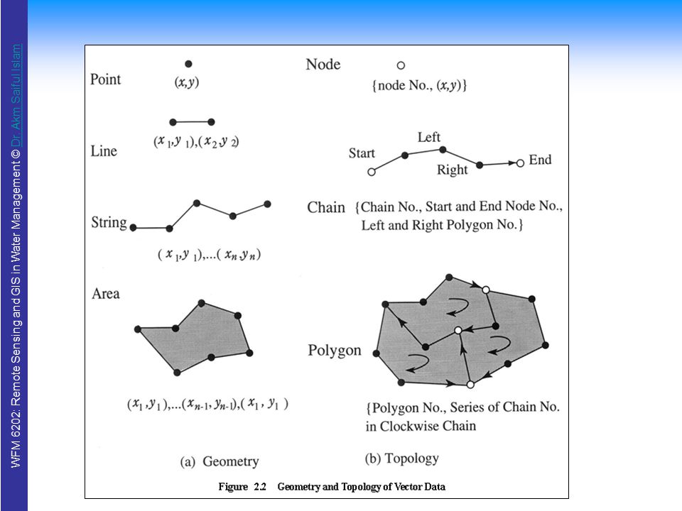
9. Vector data model: Geometry and Topology
Spatial objects are classified into
point object such as meteorological station,
line object such as highway and
area object such as agricultural land,
which are represented geometrically by point, line and area respectively
Topology
refers to the relationships or connectivity between spatial objects

10. Geometry of Vector Data
- is given by point, line and area objects
Node
an intersect of more than two lines or strings, or start and end point of string with node number
Chain
a line or a string with chain number, start and end node number, left and right neighbored polygons
Polygon
an area with polygon number, series of chains that form the area in clockwise order (minus sign is assigned in case of anti-clockwise order).

11. Topological of Vector data
Relationship between nodes and chains, the following topology should be built.
Chain : Chain ID, Start Node ID, End Node ID, Attributes.
Node: Node ID, (x, y), adjacent chain IDs (positive for to node, negative for from node).
For relationship between polygons the following additional topology need to be built
Chain geometry : Chain ID, Start Coordinates, Point Coordinates, End Coordinates.
Chain topology : Chain ID, Start Node ID, End Node ID, Left Polygon ID, Right Polygon ID, (Attributes).
Polygon topology : Polygon ID, Series of Chain ID, in clockwise order (Attributes).

13. The data structure of a point coverage
Point List ID
x, y 1
2,9 2
4,4 3
2,2 4
6,2

14. Building Topology: (See also Figure 3.9)

15. Assignment-1 Find the of Figure 3.9 Submitted by next class
Topology of node
Topology of chain
Topology of polygon
Chain geometry
Submitted by
next class c

16. Arc# L-poly R-poly 1 100 101 2 102 3 103 4 5 6 7 104 Arc#
x,y coordinates 1
(1,3) (1,9) (4,9) 2
(4,9) (9,9) (9,6) 3
(9,6) (9,1) (1,1) (1,3) 4
(4,9) (4,7) (5,5) (5,3) 5
(9,6) (7,3) (5,3) 6
(5,3) (1,3) 7
(5,7) (6,8) (7,7) (7,6) (5,6) (5,7)
Arc-coordinate list
Left/right list
Polygon #
Arc #
101
1,4,6
102
4,2,5,0,7
103
6,5,3
104 7
Figure 3.9
Polygon/Arc List

17. Topological Relationships between Spatial Objects

18. Geometry of Raster Data
- is given by point, line and area objects
Point objects A point is given by point ID, coordinates (i, j) and the attributes
Line object A line is given by line ID, series of coordinates forming the line, and the attributes
Area objects An area segment is given by area ID, a group of coordinates forming the area and the attributes.

19. Topological features of Raster Data
- One of the weak points in raster model is the difficulty in network and spatial analysis as compared with vector model.
Boundary
Boundary is defined as 2 x 2 pixel window that has two different classes
Node
A node in polygon model can be defined as a 2 x 2 window that has more than three different classes

20. Example of
Raster boundary

21. Attributes
Attributes are often termed "thematic data" or "non-spatial data", that are linked with spatial data or geometric data.
An attribute has a defined characteristic of entity in the real world.
Attribute can be categorized as normal, ordinal, numerical, conditional and other characteristics.
Attribute values are often listed in attribute tables which will establish relationships between the attributes and spatial data such as point, line and area objects, and also among the attributes

22. Layers
Spatial objects in digital representation can be grouped into layers.
For example, a map can be divided into a set of map layers consisting of contours, boundaries, roads, rivers, houses, forests etc.
Map Layers

23. Overlay of Spatial data layers
Two different object layers can be overlaid which can result another layers

24. ESRI’s models
Shapefiles – as non-topological data format. Shape file treats points are pair of x, y coordinates, a line as a series of points and a polygon as a series of lines.
Can be displayed more rapidly on monitors.
Interoperable among other software.
Coverage – as topological based vector data format. A coverage can be point coverage, line coverage or polygon coverage.
Connectivity: Arcs connect to each other at nodes.
Area definition: An area is defined by a series of connected arcs.
Contiguity: Arcs have directions and left and right polygons

25. Data models for composite features
TIN – Triangulated irregular network data model approximates the terrain with a set of non-overlapping triangles.
Regions – is defined here as a geographic area with similar characteristics. A coverage feature class that can represent a single area feature as more than one polygon.
Routes - is a line feature such as highway, a bike path, or a stream but unlike other linear features, a route has a measurement system that allows linear measures to be used on a projected coordinate system.

26. Triangulated Irregular Network (TIN)
Triangulated irregular network. A vector data structure used to store and display surface models.
A TIN partitions geographic space using a set of irregularly spaced data points, each of which has an x-, y-, and z-value.
These points are connected by edges into a set of contiguous, non-overlapping triangles, creating a continuous surface that represents the terrain.
TIN
TIN & Contour

27. Components of TIN Nodes Edges Triangles Hull
The nodes originate from the points and line vertices contained in the input data sources. Every node is incorporated in the TIN triangulation. Every node in the TIN surface model must have a z value.
Every node is joined with its nearest neighbors by edges to form triangles which satisfy the Delaunay criterion. Each edge has two nodes, but a node may have two or more edges. Because edges have a node with a z value at each end, it is possible to calculate a slope along the edge from one node to the other.
Each triangular facet describes the behavior of a portion of the TIN's surface. The x,y,z coordinate values of a triangle’s three nodes can be used to derive information about the facet, such as slope, aspect, surface area, and surface length.
The hull of a TIN is formed by one or more polygons containing the entire set of data points used to construct the TIN. The hull polygons define the zone of interpolation of the TIN. Inside or on the edge of the hull polygons, it is possible to interpolate surface z values, perform analysis, and generate surface displays. Outside the hull polygons, it is not possible to derive information about the surface. The hull of a TIN can be formed by one or more polygons which can be non-convex.
Nodes
Edges
Triangles
Hull

28. Delaunay Triangulation for TIN
A method of fitting triangles to a set of points. The triangles are defined by the condition that the circumscribing circle of any triangle does not contain any other points of the data except the three defining it.
It is a method which produces triangles with a low variance in edge length. The resulting triangles may be used as an irregular tessellation for interpolation of other points on a surface.

29. Region and polygon -1
Polygons do not overlap and completely cover the area being represented (do not contain any void areas).
In a region, the polygons representing geographic features can be freestanding, they can overlap, and they need not exhaust the total area.

30. Region and polygon -2
Another premise of polygons is that each geographic feature is represented by one polygon.
This is extended for regions, so that a single geographic feature can be represented by several polygons.

31. Region and polygon -3
As with points, lines, and polygons, each region is given a unique identifier. As with polygons, area and perimeter are maintained for each region.
Constructing regions with polygons is similar to constructing polygons from arcs. Whereas a polygon is a list of arcs, a region is simply a list of polygons. One important distinction exists: the order of the polygons is not significant.

32. Route
In ArcGIS, the term route refers to any linear feature, such as a city street, highway, river, or pipe, that has a unique identifier and a common measurement system along each linear feature.
A collection of routes with a common measurement system is a route feature class. Each route in the feature class will also have a unique identifier. Line features with the same unique identifier are considered to be part of the same route:
Route feature classes are created and managed as line feature classes in the geodatabase. You can also use route feature classes from ArcInfo coverages and polyline shapefiles that include route identifiers and measured features.

33. Point events along Route
Point events occur at a precise point location along a route. Accident locations along highways, signals along rail lines, bus stops along bus routes, Wells or gauging stations along river reaches, pumping stations along pipe lines, Manholes along city streets and valves along pipes are all examples of point events. Point events use a single measure value to describe their location.

34. Line events along Route
Line events describe portions of routes. Pavement quality, salmon spawning grounds, bus fares, pipe widths, and traffic volumes are all examples of line events. Line events use two measure values to describe their location.

35. Polygon events along Route
Locating polygon features along routes computes the route and measure information at the geometric intersection of polygon data and route data. Once polygon data has been located along routes, the resulting event table can be used, for example, to calculate the length of route that traveled through each polygon.
Examples:
Soils, spillways, areas of inundation, or hazard zones along river reaches
Wetlands, hazard zones, or town boundaries along highways

36. Example of Route
Hydrologists and ecologists use linear referencing on stream networks to locate various types of events
The route feature class for streams provides measures along the streams using river reach mile.
Point and line event tables record the route ID and location along each river reach.
These event tables can be used to locate point and line events.

37. Route system
A collection of routes with a common system of measurement is called a route system. Route systems usually define linear features with similar attributes. For example, a set of all bus routes in a county would be a route system.
Many route systems can exist within a single coverage. For example, school bus, truck, and ambulance route systems could exist in a coverage of a city.
Route systems are built using arcs, routes, and sections, and can accurately model linear features without having to modify the underlying arc-node topology.
The route below is defined using four arcs. Notice how the route's endpoints fall along the arcs. Routes need not begin and end at nodes.
Sections, as shown below, are the arcs or portions of arcs used to define each route. They form the infrastructure of the route system.
The diagram below shows an example of attributes containing distance measurements, such as milepost numbers or addresses, which can be used to locate events, such as accidents or pavement quality.

38. Dynamic segmentation
Dynamic segmentation (DynSeg) is the process of computing the map location (shape) of events stored in an event table.
Dynamic segmentation is what allows multiple sets of attributes to be associated with any portion of a linear feature.