Download presentation
Presentation is loading. Please wait.

1
Phylogeny Tree Reconstruction 1 4 3 2 5 1 4 2 3 5

2
Inferring Phylogenies Trees can be inferred by several criteria: Morphology of the organisms Sequence comparison Example: Orc: ACAGTGACGCCCCAAACGT Elf: ACAGTGACGCTACAAACGT Dwarf: CCTGTGACGTAACAAACGA Hobbit: CCTGTGACGTAGCAAACGA Human: CCTGTGACGTAGCAAACGA

3
Modeling Evolution During infinitesimal time t, there is not enough time for two substitutions to happen on the same nucleotide So we can estimate P(x | y, t), for x, y {A, C, G, T} Then let P(A|A, t) …… P(A|T, t) S( t) = ……… P(T|A, t) ……P(T|T, t) xx y tt
, for x, y {A, C, G, T} Then let P(A|A, t) …… P(A|T, t) S( t) = ……… P(T|A, t) ……P(T|T, t) xx y tt")
4
Modeling Evolution Reasonable assumption: multiplicative (implying a stationary Markov process) S(t+t’) = S(t)S(t’) That is, P(x | y, t+t’) = z P(x | z, t) P(z | y, t’) Jukes-Cantor: constant rate of evolution 1 - 3 For short time , S( ) = I+R = 1 - 3 1 - 3 1 - 3 AC GT
 S(t+t’) = S(t)S(t’) That is, P(x | y, t+t’) = z P(x | z, t) P(z | y, t’) Jukes-Cantor: constant rate of evolution For short time , S( ) = I+R = AC GT")
5
Modeling Evolution Jukes-Cantor: For longer times, r(t)s(t) s(t) s(t) S(t) = s(t)r(t) s(t) s(t) s(t)s(t) r(t) s(t) s(t)s(t) s(t) r(t) Where we can derive: r(t) = ¼ (1 + 3 e -4 t ) s(t) = ¼ (1 – e -4 t ) S(t+ ) = S(t)S( ) = S(t)(I + R ) Therefore, (S(t+ ) – S(t))/ = S(t) R At the limit of 0, S’(t) = S(t) R Equivalently, r’ = -3 r + 3 s s’ = - s + r Those diff. equations lead to: r(t) = ¼ (1 + 3 e -4 t ) s(t) = ¼ (1 – e -4 t )
 = ¼ (1 + 3 e -4 t ) s(t) = ¼ (1 – e -4 t ).")
6
Modeling Evolution Kimura: Transitions: A/G, C/T Transversions: A/T, A/C, G/T, C/G Transitions (rate ) are much more likely than transversions (rate ) r(t)s(t) u(t) s(t) S(t) = s(t)r(t) s(t) u(t) u(t)s(t) r(t) s(t) s(t)u(t) s(t) r(t) Wheres(t) = ¼ (1 – e -4 t ) u(t) = ¼ (1 + e -4 t – e -2( + )t ) r(t) = 1 – 2s(t) – u(t)
 are much more likely than transversions (rate ) r(t)s(t) u(t) s(t) S(t) = s(t)r(t) s(t) u(t) u(t)s(t) r(t) s(t) s(t)u(t) s(t) r(t) Wheres(t) = ¼ (1 – e -4 t ) u(t) = ¼ (1 + e -4 t – e -2( + )t ) r(t) = 1 – 2s(t) – u(t)")
7
Phylogeny and sequence comparison Basic principles: Degree of sequence difference is proportional to length of independent sequence evolution Only use positions where alignment is pretty certain – avoid areas with (too many) gaps
 gaps")
8
Distance between two sequences Given sequences x i, x j, Define d ij = distance between the two sequences One possible definition: d ij = fraction f of sites u where x i [u] x j [u] Better model (Jukes-Cantor): f = ¾ (1 – e -4 t ) ¾ e -4 t = ¾ - f log (e -4 t ) = log (1 – 4/3 f) d ij = t = - ¼ -1 log(1 – 4/3 f)
![Distance between two sequences Given sequences x i, x j, Define d ij = distance between the two sequences One possible definition: d ij = fraction f of sites u where x i [u] x j [u] Better model (Jukes-Cantor): f = ¾ (1 – e -4 t ) ¾ e -4 t = ¾ - f log (e -4 t ) = log (1 – 4/3 f) d ij = t = - ¼ -1 log(1 – 4/3 f)](http://images.slideplayer.com/16/4976723/slides/slide_8.jpg "Distance between two sequences Given sequences x i, x j, Define d ij = distance between the two sequences One possible definition: d ij = fraction f of sites u where x i [u] x j [u] Better model (Jukes-Cantor): f = ¾ (1 – e -4 t ) ¾ e -4 t = ¾ - f log (e -4 t ) = log (1 – 4/3 f) d ij = t = - ¼ -1 log(1 – 4/3 f)")
9
A simple clustering method for building tree UPGMA (unweighted pair group method using arithmetic averages) Or the Average Linkage Method Given two disjoint clusters C i, C j of sequences, 1 d ij = ––––––––– {p Ci, q Cj} d pq |C i | |C j | Claim that if C k = C i C j, then distance to another cluster C l is: d il |C i | + d jl |C j | d kl = –––––––––––––– |C i | + |C j | Proof Ci,Cl d pq + Cj,Cl d pq d kl = –––––––––––––––– (|C i | + |C j |) |C l | |C i |/(|C i ||C l |) Ci,Cl d pq + |C j |/(|C j ||C l |) Cj,Cl d pq = –––––––––––––––––––––––––––––––––––– (|C i | + |C j |) |C i | d il + |C j | d jl = ––––––––––––– (|C i | + |C j |)
 Or the Average Linkage Method Given two disjoint clusters C i, C j of sequences, 1 d ij = ––––––––– {p Ci, q Cj} d pq |C i | |C j | Claim that if C k = C i C j, then distance to another cluster C l is: d il |C i | + d jl |C j | d kl = –––––––––––––– |C i | + |C j | Proof Ci,Cl d pq + Cj,Cl d pq d kl = –––––––––––––––– (|C i | + |C j |) |C l | |C i |/(|C i ||C l |) Ci,Cl d pq + |C j |/(|C j ||C l |) Cj,Cl d pq = –––––––––––––––––––––––––––––––––––– (|C i | + |C j |) |C i | d il + |C j | d jl = ––––––––––––– (|C i | + |C j |)")
10
Algorithm: Average Linkage Initialization: Assign each x i into its own cluster C i Define one leaf per sequence, height 0 Iteration: Find two clusters C i, C j s.t. d ij is min Let C k = C i C j Define node connecting C i, C j, & place it at height d ij /2 Delete C i, C j Termination: When two clusters i, j remain, place root at height d ij /2 1 4 3 2 5 1 4 2 3 5

11
Example vwxyz v 06888 w 0888 x 044 y 02 z 0 yzxwv 1 2 3 4 vwxyz v 0688 w 088 x 04 0 vwxyz v 068 w 08 0 vwxyz vw 08 xyz 0

12
Ultrametric Distances and Molecular Clock Definition: A distance function d(.,.) is ultrametric if for any three distances d ij d ik d ij, it is true that d ij d ik = d ij The Molecular Clock: The evolutionary distance between species x and y is 2 the Earth time to reach the nearest common ancestor That is, the molecular clock has constant rate in all species 14235 years The molecular clock results in ultrametric distances
 is ultrametric if for any three distances d ij d ik d ij, it is true that d ij d ik = d ij The Molecular Clock: The evolutionary distance between species x and y is 2 the Earth time to reach the nearest common ancestor That is, the molecular clock has constant rate in all species years The molecular clock results in ultrametric distances")
13
Ultrametric Distances & Average Linkage Average Linkage is guaranteed to reconstruct correctly a binary tree with ultrametric distances Proof: Exercise (extra credit) 1423 5
")
14
Weakness of Average Linkage Molecular clock: all species evolve at the same rate (Earth time) However, certain species (e.g., mouse, rat) evolve much faster Example where UPGMA messes up: 2 3 4 1 1 4 3 2 Correct tree AL tree
 However, certain species (e.g., mouse, rat) evolve much faster Example where UPGMA messes up: Correct tree AL tree")
15
Additive Distances Given a tree, a distance measure is additive if the distance between any pair of leaves is the sum of lengths of edges connecting them Given a tree T & additive distances d ij, can uniquely reconstruct edge lengths: Find two neighboring leaves i, j, with common parent k Place parent node k at distance d km = ½ (d im + d jm – d ij ) from any node m 1 2 3 4 5 6 7 8 9 10 12 11 13 d 1,4
 from any node m d 1,4")
16
Additive Distances For any four leaves x, y, z, w, consider the three sums d(x, y) + d(z, w) d(x, z) + d(y, w) d(x, w) + d(y, z) One of them is smaller than the other two, which are equal d(x, y) + d(z, w) < d(x, z) + d(y, w) = d(x, w) + d(y, z) x y z w
 + d(z, w) d(x, z) + d(y, w) d(x, w) + d(y, z) One of them is smaller than the other two, which are equal d(x, y) + d(z, w) < d(x, z) + d(y, w) = d(x, w) + d(y, z) x y z w")
17
Reconstructing Additive Distances Given T x y z w v 5 4 7 3 3 4 6 vwxyz v 0101716 w 01514 x 0915 y 014 z 0 T If we know T and D, but do not know the length of each leaf, we can reconstruct those lengths D

18
Reconstructing Additive Distances Given T x y z w v vwxyz v 0101716 w 01514 x 0915 y 014 z 0 T D

19
Reconstructing Additive Distances Given T x y z w v vwxyz v 0101716 w 01514 x 0915 y 014 z 0 T D axyz a 01110 x 0915 y 014 z 0 a D1D1 d ax = ½ (d vx + d wx – d vw ) d ay = ½ (d vy + d wy – d vw ) d az = ½ (d vz + d wz – d vw )
 d ay = ½ (d vy + d wy – d vw ) d az = ½ (d vz + d wz – d vw )")
20
Reconstructing Additive Distances Given T x y z w v T axyz a 01110 x 0915 y 014 z 0 a D1D1 abz a 0610 b 0 z 0 D2D2 b c ac a 03 c 0 D3D3 d(a, c) = 3 d(b, c) = d(a, b) – d(a, c) = 3 d(c, z) = d(a, z) – d(a, c) = 7 d(b, x) = d(a, x) – d(a, b) = 5 d(b, y) = d(a, y) – d(a, b) = 4 d(a, w) = d(z, w) – d(a, z) = 4 d(a, v) = d(z, v) – d(a, z) = 6 Correct!!! 5 4 7 3 3 4 6

21
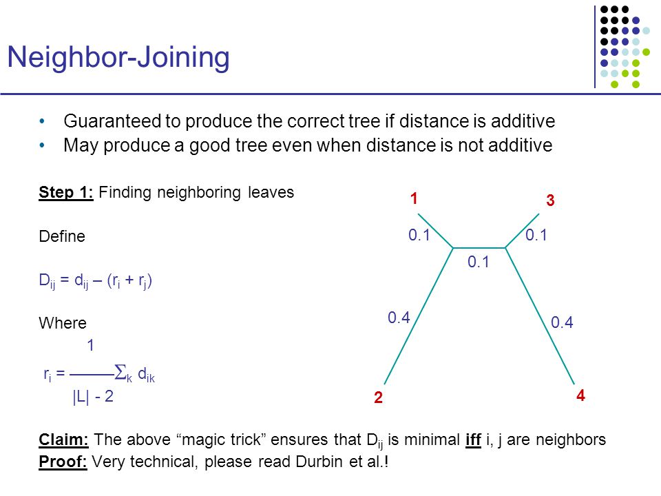
Neighbor-Joining Guaranteed to produce the correct tree if distance is additive May produce a good tree even when distance is not additive Step 1: Finding neighboring leaves Define D ij = d ij – (r i + r j ) Where 1 r i = ––––– k d ik |L| - 2 Claim: The above “magic trick” ensures that D ij is minimal iff i, j are neighbors Proof: Very technical, please read Durbin et al.! 1 2 4 3 0.1 0.4
22
Algorithm: Neighbor-joining Initialization: Define T to be the set of leaf nodes, one per sequence Let L = T Iteration: Pick i, j s.t. D ij is minimal Define a new node k, and set d km = ½ (d im + d jm – d ij ) for all m L Add k to T, with edges of lengths d ik = ½ (d ij + r i – r j ) Remove i, j from L; Add k to L Termination: When L consists of two nodes, i, j, and the edge between them of length d ij
 for all m L Add k to T, with edges of lengths d ik = ½ (d ij + r i – r j ) Remove i, j from L; Add k to L Termination: When L consists of two nodes, i, j, and the edge between them of length d ij.")
23
Parsimony One of the most popular methods Idea: Find the tree that explains the observed sequences with a minimal number of substitutions Two computational subproblems: 1.Find the parsimony cost of a given tree (easy) 2.Search through all tree topologies (hard)
 2.Search through all tree topologies (hard)")
24
Parsimony Scoring Given a tree, and an alignment column u Label internal nodes to minimize the number of required substitutions Initialization: Set cost C = 0; k = 2N – 1 Iteration: If k is a leaf, set R k = { x k [u] } If k is not a leaf, Let i, j be the daughter nodes; Set R k = R i R j if intersection is nonempty Set R k = R i R j, and C += 1, if intersection is empty Termination: Minimal cost of tree for column u, = C
![Parsimony Scoring Given a tree, and an alignment column u Label internal nodes to minimize the number of required substitutions Initialization: Set cost C = 0; k = 2N – 1 Iteration: If k is a leaf, set R k = { x k [u] } If k is not a leaf, Let i, j be the daughter nodes; Set R k = R i R j if intersection is nonempty Set R k = R i R j, and C += 1, if intersection is empty Termination: Minimal cost of tree for column u, = C](http://images.slideplayer.com/16/4976723/slides/slide_24.jpg "Parsimony Scoring Given a tree, and an alignment column u Label internal nodes to minimize the number of required substitutions Initialization: Set cost C = 0; k = 2N – 1 Iteration: If k is a leaf, set R k = { x k [u] } If k is not a leaf, Let i, j be the daughter nodes; Set R k = R i R j if intersection is nonempty Set R k = R i R j, and C += 1, if intersection is empty Termination: Minimal cost of tree for column u, = C")
25
Example A B A B {A, B} C+=1 {A, B} C+=1 {A} {B} {A} {B}

26
Example AAAB {A} {B} BABA {A}{B}{A}{B} {A} {A,B} {B}

27
Traceback: 1.Choose an arbitrary nucleotide from R 2N – 1 for the root 2.Having chosen nucleotide r for parent k, If r R i choose r for daughter i Else, choose arbitrary nucleotide from R i Easy to see that this traceback produces some assignment of cost C Traceback to find ancestral nucleotides

28
Example A B A B {A, B} {A} {B} {A} {B} A B A B A A A x x A B A B A B A x x A B A B B B B x x Admissible with Traceback Still optimal, but inadmissible with Traceback

29
Number of labeled unrooted tree topologies How many possibilities are there for leaf 4? 1 2 3 4 4 4

30
Number of labeled unrooted tree topologies How many possibilities are there for leaf 4? For the 4 th leaf, there are 3 possibilities 1 2 3 4

31
Number of labeled unrooted tree topologies How many possibilities are there for leaf 5? For the 5 th leaf, there are 5 possibilities 1 2 3 4 5

32
Number of labeled unrooted tree topologies How many possibilities are there for leaf 6? For the 6 th leaf, there are 7 possibilities 1 2 3 4 5

33
Number of labeled unrooted tree topologies How many possibilities are there for leaf n? For the n th leaf, there are 2n – 5 possibilities 1 2 3 4 5

34
Number of labeled unrooted tree topologies #unrooted trees for n taxa: (2n-5)*(2n-7)*...*3*1 = (2n-5)! / [2n-3*(n-3)!] #rooted trees for n taxa: (2n-3)*(2n-5)*(2n-7)*...*3 = (2n-3)! / [2n-2*(n-2)!] 1 2 3 4 5 N = 10 #unrooted: 2,027,025 #rooted: 34,459,425 N = 30 #unrooted: 8.7x10 36 #rooted: 4.95x10 38
!] #rooted trees for n taxa: (2n-3)*(2n-5)*(2n-7)*...*3 = (2n-3). / [2n-2*(n-2)!] N = 10 #unrooted: 2,027,025 #rooted: 34,459,425 N = 30 #unrooted: 8.7x10 36 #rooted: 4.95x")
35
Search through tree topologies: Branch and Bound Observation: adding an edge to an existing tree can only increase the parsimony cost Enumerate all unrooted trees with at most n leaves: [i 3 ][i 5 ][i 7 ]……[i 2N–5] ] where each i k can take values from 0 (no edge) to k At each point keep C = smallest cost so far for a complete tree Start B&B with tree [1][0][0]……[0] Whenever cost of current tree T is > C, then: T is not optimal Any tree extending T with more edges is not optimal: Increment by 1 the rightmost nonzero counter
![Search through tree topologies: Branch and Bound Observation: adding an edge to an existing tree can only increase the parsimony cost Enumerate all unrooted trees with at most n leaves: [i 3 ][i 5 ][i 7 ]……[i 2N–5] ] where each i k can take values from 0 (no edge) to k At each point keep C = smallest cost so far for a complete tree Start B&B with tree [1][0][0]……[0] Whenever cost of current tree T is > C, then: T is not optimal Any tree extending T with more edges is not optimal: Increment by 1 the rightmost nonzero counter](http://images.slideplayer.com/16/4976723/slides/slide_35.jpg "Search through tree topologies: Branch and Bound Observation: adding an edge to an existing tree can only increase the parsimony cost Enumerate all unrooted trees with at most n leaves: [i 3 ][i 5 ][i 7 ]……[i 2N–5] ] where each i k can take values from 0 (no edge) to k At each point keep C = smallest cost so far for a complete tree Start B&B with tree [1][0][0]……[0] Whenever cost of current tree T is > C, then: T is not optimal Any tree extending T with more edges is not optimal: Increment by 1 the rightmost nonzero counter")
36
Bootstrapping to get the best trees Main outline of algorithm 1.Select random columns from a multiple alignment – one column can then appear several times 2.Build a phylogenetic tree based on the random sample from (1) 3.Repeat (1), (2) many (say, 1000) times 4.Output the tree that is constructed most frequently
 3.Repeat (1), (2) many (say, 1000) times 4.Output the tree that is constructed most frequently")
37
Probabilistic Methods A more refined measure of evolution along a tree than parsimony P(x 1, x 2, x root | t 1, t 2 ) = P(x root ) P(x 1 | t 1, x root ) P(x 2 | t 2, x root ) If we use Jukes-Cantor, for example, and x 1 = x root = A, x 2 = C, t 1 = t 2 = 1, = p A ¼(1 + 3e -4α ) ¼(1 – e -4α ) = (¼) 3 (1 + 3e -4α )(1 – e -4α ) x1x1 t2t2 x root t1t1 x2x2
 = P(x root ) P(x 1 | t 1, x root ) P(x 2 | t 2, x root ) If we use Jukes-Cantor, for example, and x 1 = x root = A, x 2 = C, t 1 = t 2 = 1, = p A ¼(1 + 3e -4α ) ¼(1 – e -4α ) = (¼) 3 (1 + 3e -4α )(1 – e -4α ) x1x1 t2t2 x root t1t1 x2x2")
38
Probabilistic Methods If we know all internal labels x u, P(x 1, x 2, …, x N, x N+1, …, x 2N-1 | T, t) = P(x root ) j root P(x j | x parent(j), t j, parent(j) ) Usually we don’t know the internal labels, therefore P(x 1, x 2, …, x N | T, t) = x N+1 x N+2 … x 2N-1 P(x 1, x 2, …, x 2N-1 | T, t) x root x1x1 x2x2 xNxN xuxu
 = P(x root ) j root P(x j | x parent(j), t j, parent(j) ) Usually we don’t know the internal labels, therefore P(x 1, x 2, …, x N | T, t) = x N+1 x N+2 … x 2N-1 P(x 1, x 2, …, x 2N-1 | T, t) x root x1x1 x2x2 xNxN xuxu")
39
Felsenstein’s Likelihood Algorithm To calculate P(x 1, x 2, …, x N | T, t) Initialization: Set k = 2N – 1 Recursion: Compute P(L k | a) for all a If k is a leaf node: Set P(L k | a) = 1(a = x k ) If k is not a leaf node: 1. Compute P(L i | b), P(L j | b) for all b, for daughter nodes i, j 2. Set P(L k | a) = b, c P(b | a, t i )P(L i | b) P(c | a, t j ) P(L j | c) Termination: Likelihood at this column = P(x 1, x 2, …, x N | T, t) = a P(L 2N-1 | a)P(a)
, P(L j | b) for all b, for daughter nodes i, j 2. Set P(L k | a) = b, c P(b | a, t i )P(L i | b) P(c | a, t j ) P(L j | c) Termination: Likelihood at this column = P(x 1, x 2, …, x N | T, t) = a P(L 2N-1 | a)P(a).")
40
Probabilistic Methods Given M (ungapped) alignment columns of N sequences, Define likelihood of a tree: L(T, t) = P(Data | T, t) = m=1…M P(x 1m, …, x nm, T, t) Maximum Likelihood Reconstruction: Given data X = (x ij ), find a topology T and length vector t that maximize likelihood L(T, t)
 alignment columns of N sequences, Define likelihood of a tree: L(T, t) = P(Data | T, t) = m=1…M P(x 1m, …, x nm, T, t) Maximum Likelihood Reconstruction: Given data X = (x ij ), find a topology T and length vector t that maximize likelihood L(T, t)")
Similar presentations
 Lecture 13 Based on: Durbin et al 7.4, Gusfield 17.1-17.3, Setubal&Meidanis 6.1.>")


 Lecture 13 Based on: Durbin et al 7.4, Gusfield 17.1-17.3, Setubal&Meidanis 6.1.>")


 Modified by Benny Chor, from slides by Shlomo Moran and Ydo Wexler (IIT)>")


 Cetacea (whales, dolphins, porpoises)>")
 Parameter Estimation with applications to inferring phylogenetic trees Comput. Genomics, lecture 7a Presentation partially taken.>")