1. I corsi vengono integrati e conterranno grosso modo due moduli:
SB: systems biology
ML: machine learning
Alternativa 1
Alternativa 2
Mattina (Fariselli)
Pomeriggio (Martelli)
Lun 1 Ott
SVM (ML)
Grafi (SB)
Mar 2 Ott
System Biology (SB)
Probabilita (ML)
Mer 3 Ott
HMM (ML)
Ven 5 Ott
Lun 8 Ott
Mar 9 Ott
Linux
Linux e python
Mer 10 Ott
Esercitazione su SVM
Gio 11 Ott
Esercitazione su HMM

2. Systems Biology. What Is It?
A branch of science that seeks to integrate
different levels of information to understand
how biological systems function.
L. Hood: “Systems biology defines and analyses
the interrelationships of all of the elements in a
functioning system in order to understand how the
system works.”
It is not (only) the number and properties of system elements but their relations!!

3. More on Systems Biology
Essence of living systems is flow of mass,
energy, and information in space and time.
The flow occurs along specific networks
Flow of mass and energy (metabolic networks)
Flow of information involving DNA (transcriptional
regulation networks)
Flow of information not involving DNA (signaling networks)
The Goal of Systems Biology:
To understand the flow of mass, energy,
and information in living systems.

4. Networks and the Core Concepts of Systems Biology
Complexity emerges at all levels of the
hierarchy of life
System properties emerge from interactions
of components
(iii) The whole is more than the sum of the parts.
(iv) Applied mathematics provides approaches to
modeling biological systems.

5. How to Describe a System
As a Whole?
Networks - The Language
of Complex Systems

6. Air Transportation Network

7. The World Wide Web

8. Fragment of a Social Network
(Melburn, 2004)
Friendship among 450 people in Canberra

9. Biological Networks A. Intra-Cellular Networks
Protein interaction networks
Metabolic Networks
Signaling Networks
Gene Regulatory Networks
Composite networks
Networks of Modules, Functional Networks Disease networks
B. Inter-Cellular Networks
Neural Networks
C. Organ and Tissue Networks
D. Ecological Networks
E. Evolution Network

10. The Protein Interaction Network of Yeast
Yeast two hybrid
Uetz et al, Nature 2000

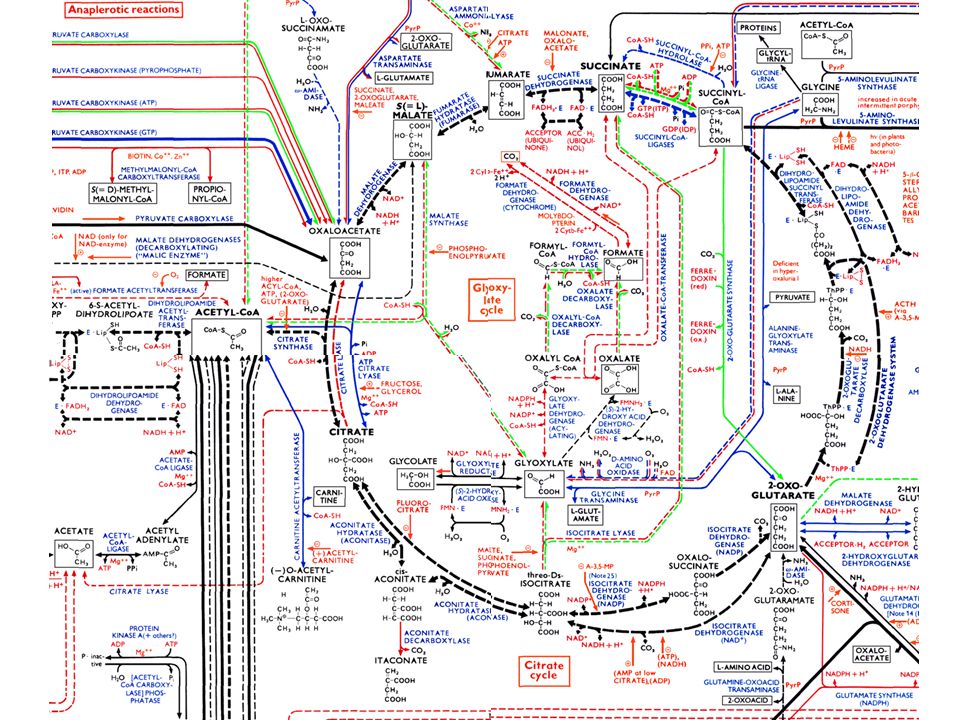
11. Metabolic Networks
Source: ExPASy

13. Gene Regulation Networks

14. _ _ _ _ _ _ _ _ _ _ _ _ _ _ _ _ _ _ _ _ _
L-A Barabasi
GENOME
miRNA
regulation?
_ _ _ _ _ _ _ _ _ _ _ _ _ _ _ _ _ _ _ _ _
PROTEOME
- -
protein-gene interactions
protein-protein interactions
Citrate Cycle
METABOLISM
Bio-chemical reactions

15. Functional Networks
Yeast: 1400 proteins, 232 complexes, nine functional groups of complexes
Number of shared proteins 20
125 55
740 43
221 33
419 28
692 12
160
147 7 83 65 41 49
172 75
321 24
260 11
596 35
103
Cell Cycle
Cell Polarity & Structure
Intermediate
and Energy
Metabolism
Protein Synthesis
and Turnover
Protein RNA / Transport
RNA
Signaling
Transcription/DNA
Maintenance/Chromatin
Structure
Number of protein complexes
Number of proteins 13
111 8 61 25 40 77 19 14 97 30 16 27
299 53 37 15 22
187 73 94
Membrane
Biogenesis &
Turnover
(Data A.-M. Gavin
et al. (2002) Nature
415, )
D. Bonchev, Chemistry & Biodiversity 1(2004)

16. What is a Network? Network is a mathematical structure
composed of points connected by lines
Network Theory <-> Graph Theory
Network  Graph
Nodes  Vertices (points)
Links  Edges (Lines)
A network can be build for any functional system
System vs. Parts = Networks vs. Nodes

17. The 7 bridges of Königsberg
The question is whether it is possible to walk with a route that crosses each bridge exactly once.

18. The representation of Euler
In 1736 Leonhard Euler formulated the problem in terms of abstracted the case of Königsberg:
by eliminating all features except the landmasses and the bridges connecting them;
by replacing each landmass with a dot (vertex) and each bridge with a line (edge).
The shape of a graph may be distorted in any way without changing the graph itself, so long as the links between nodes are unchanged. It does not matter whether the links are straight or curved, or whether one node is to the left or right of another.

19. The solution depends on the node degree3
In a continuous path crossing the edges exactly once, each visited node requires an edge for entering and a different edge for exiting (except for the start and the end nodes). 5 3 3
A path crossing once each edge is called Eulerian path.
It possible IF AND ONLY IF there are exactly two or zero nodes of odd degree.
Since the graph corresponding to Königsberg has four nodes of odd degree, it cannot have an Eulerian path.

20. The solution depends on the node degree3 6
End 2 4 5 1
Start
If there are two nodes of odd degree, those must be the starting and ending points of an Eulerian path.

21. Hamiltonian paths Find a path visiting each node exactly one
Conditions of existence for Hamiltonian paths are not simple

22. Hamiltonian paths

23. Graph nomenclature
Graphs can be simple or multigraphs, depending on whether
the interaction between two neighboring nodes is unique or can be multiple, respectively.
A node can have or not self loops

24. Graph nomenclature
Networks can be undirected or directed, depending on whether
the interaction between two neighboring nodes proceeds in both
directions or in only one of them, respectively.  1 2 3 4 5 6
The specificity of network nodes and links can be quantitatively
characterized by weights
2.5
7.3
3.3
12.7
5.4
8.1
2.5
Vertex-Weighted
Edge-Weighted

25. Graph nomenclature
A network can be connected (presented by a single component) or disconnected (presented by several disjoint components).
connected
disconnected
Networks having no cycles are termed trees. The more cycles thenetwork has, the more complex it is.
trees
cyclic graphs

26. Graph nomenclature
Paths
Stars
Cycles
Complete Graphs

27. Large graphs = Networks

28. Statistical features of networks
Vertex degree distribution (the degree of a vertex is the number of vertices connected with it via an edge)

29. Statistical features of networks
Clustering coefficient: the average proportion of neighbours of a vertex that are themselves neighbours
Node
4 Neighbours (N)
2 Connections among the Neighbours
6 possible connections among the Neighbours
(Nx(N-1)/2)
Clustering for the node = 2/6
Clustering coefficient: Average over all the nodes

30. Statistical features of networks
Clustering coefficient: the average proportion of neighbours of a vertex that are themselves neighbours
C=0
C=0
C=0
C=1

31. Statistical features of networks
Given a pair of nodes, compute the shortest path between them
Average shortest distance between two vertices
Diameter: maximal shortest distance
How many degrees of separation are they between two random people in the world, when friendship networks are considered?

32. How to compute the shortest path between home and work?
Edge-weighted Graph
The exaustive search can be too much time-consuming

33. The Dijkstra’s algorithm
Fixed nodes
NON –fixed nodes
Initialization:
Fix the distance between “Casa” and “Casa” equal to 0
Compute the distance between “Casa” and its neighbours
Set the distance between “Casa” and its NON-neighbours equal to ∞

34. The Dijkstra’s algorithm
Fixed nodes
NON –fixed nodes
Iteration (1):
Search the node with the minimum distance among the NON-fixed nodes and Fix its distance, memorizing the incoming direction

35. The Dijkstra’s algorithm4
Iteration (2):
Update the distance of NON-fixed nodes, starting from the fixed distances
Fixed nodes
NON –fixed nodes

36. The Dijkstra’s algorithm
Fixed nodes
NON –fixed nodes
The updated distance is different from the previous one
Iteration:
Fix the NON-fixed nodes with minimum distance
Update the distance of NON-fixed nodes, starting from the fixed distances.

37. The Dijkstra’s algorithm
Fixed nodes
NON –fixed nodes
Iteration:
Fix the NON-fixed nodes with minimum distance
Update the distance of NON-fixed nodes, starting from the fixed distances.

38. The Dijkstra’s algorithm
Fixed nodes
NON –fixed nodes
Iteration:
Fix the NON-fixed nodes with minimum distance
Update the distance of NON-fixed nodes, starting from the fixed distances.

39. The Dijkstra’s algorithm
Fixed nodes
NON –fixed nodes
Iteration:
Fix the NON-fixed nodes with minimum distance
Update the distance of NON-fixed nodes, starting from the fixed distances.

40. The Dijkstra’s algorithm
Fixed nodes
NON –fixed nodes
Iteration:
Fix the NON-fixed nodes with minimum distance
Update the distance of NON-fixed nodes, starting from the fixed distances.

41. The Dijkstra’s algorithm
Fixed nodes
NON –fixed nodes
Conclusion:
The label of each node represents the minimal distance from the starting node
The minimal path can be reconstructed with a back-tracing procedure

42. Statistical features of networks
Vertex degree distribution
Clustering coefficient
Average shortest distance between two vertices
Diameter: maximal shortest distance

43. Two reference models for networks
Regular network (lattice)
Random network (Erdös+Renyi, 1959)
Regular connections
Each edge is randomly set with probability p

44. Two reference models for networks
Comparing networks with the same number of nodes (N) and edges
Poisson distribution
Degree distribution
Exp decay
Average shortest path
≈ N
≈ log (N)
Average connectivity
high
low

45. Some examples for real networks
size
vertex degree
shortest path
Shortest path in fitted random graph
Clustering
Clustering in random graph
Film actors
225,226 61
3.65
2.99
0.79
MEDLINE coauthorship
1,520,251
18.1
4.6
4.91
0.43
1.8 x 10-4
E.Coli substrate graph
282
7.35
2.9
3.04
0.32
0.026
C.Elegans neuron network 14
2.65
2.25
0.28
0.05
Real networks are not regular (low shortest path)
Real networks are not random (high clustering)

46. Adding randomness in a regular network
Random changes in edges OR
Addition of random links

47. Adding randomness in a regular network
(rewiring)
Networks with high clustering (like regular ones) and low path length (like random ones) can be obtained:
SMALL WORLD NETWORKS (Strogatz and Watts, 1999)

48. Small World Networks
A small amount of random shortcuts can decrease the path length, still maintaining a high clustering: this model “explains” the 6-degrees of separations in human friendship network

49. What about the degree distribution in real networks?
Both random and small world models predict an approximate Poisson distribution:
most of the values are near the mean;
Exponential decay when k gets higher: P(k) ≈ e-k, for large k.

50. What about the degree distribution in real networks?
In 1999, modelling the WWW (pages: nodes; link: edges), Barabasi and Albert discover a slower than exponential decay:
P(k) ≈ k-a with 2 < a < 3, for large k

51. Scale-free networks
Networks that are characterized by a power-law degree distribution are highly non-uniform: most of the nodes have only a few links. A few nodes with a very large number of links, which are often called hubs, hold these nodes together. Networks with a power degree distribution are called scale-free
hubs
It is the same distribution of wealth following Pareto’s law:
Few people (20%) possess most of the wealth (80%), most of the people (80%) possess the rest (20%)

52. Hubs
Attacks to hubs can rapidly destroy the network

53. Three non biological scale-free networks
Note the log-log scale
LINEAR PLOT
Albert and Barabasi, Science 1999

54. How can a scale-free network emerge?
Network growth models: start with one vertex.

55. How can a scale-free network emerge?
Network growth models: new vertex attaches to existing vertices by preferential attachment: vertex tends choose vertex according to vertex degree he
In economy this is called Matthew’s effect: The rich get richer
This explain the Pareto’s distribution of wealth

56. How can a scale-free network emerge?
Network growth models: hubs emerge
(in the WWW: new pages tend to link to existing, well linked pages)

57. Metabolic pathways are scale-free
Hubs are pyruvate, coenzyme A….

58. Protein interaction networks are scale-free
Degree is in some measure related to phenotypic effect upon gene knock-out
Red : lethal
Green: non lethal
Yellow: Unknown

59. Caveat: different experiments give different results
Titz et al, Exp Review Proteomics, 2004

60. How can a scale-free network emerge?
Gene duplication (and differentiation): duplicated genes give origin to a protein that interacts with the same proteins as the original protein (and then specializes its functions)

61. Caveat on the use of the scale-free theory
The same noisy data can be fitted in different ways
A sub-net of a non-free-scale network can have a scale-free behaviour
Finding a scale-free behaviour do NOT imply the growth with preferential attachment mechanism
Keller, BioEssays 2006

62. Hierarchical networks
Standard free scale models have low clustering: a modular hierarchical model accounts for high clustering, low average path and scale-freeness

63. Modules Sub-graphs more represented than expected
209 bi-fan motifs found in the E.coli regulatory network

64. Summary Many complex networks in nature and technology
have common features.
They differ considerably from random networks
of the same size
By studying network structure and dynamics, and
by using comparative network analysis, one can
get answers of important biological questions.

65. Fundamental Biological Questions to Answer
(i) Which interactions and groups of interactions are likely to have
equivalent functions across species?
(ii) Based on these similarities, can we predict new functional
information about proteins and interactions that are poorly
characterized?
(iii) What do these relationships tell us about the evolution of proteins,
networks and whole species?
(iv) How to reduce the noise in biological data: Which interactions
represent true binding events?
False-positive interaction is unlikely to be reproduced across the
interaction maps of multiple species.
Fundamental Biological
Questions to Answer
(i) Which interactions and groups of interactions are likely
to have equivalent functions across species?
(ii) Based on these similarities, can we predict new functional
information about proteins and interactions that are poorly
characterized?
(iii) What do these relationships tell us about the
evolution of proteins, networks and whole species?
(iv) How to reduce the noise in biological data: Which
interactions represent true binding events?
False-positive interaction is unlikely to be reproduced
across the interaction maps of multiple species.

66. Barabasi and Oltvai (2004) Network Biology: understanding the cell’s functional organization. Nature Reviews Genetics 5:
Stogatz (2001) Exploring complex networks. Nature 410:
Hayes (2000) Graph theory in practice. American Scientist 88:9-13/
Mason and Verwoerd (2006) Graph theory and networks in Biology
Keller (2005) Revisiting scale-free networks. BioEssays 27.10: