1. Music Physics 202 Professor Vogel (Professor Carkner’s notes, ed) Lecture 9

2. Music  A musical instrument is a device for setting up standing waves of known frequency  A standing wave oscillates with large amplitude and so is loud  We shall consider an generalized instrument consisting of a pipe which may be open at one or both ends  Like a pipe organ or a saxophone  There will always be a node at the closed end and an anti-node at the open end  Can have other nodes or antinodes in between, but this rule must be followed  Closed end is like a tied end of string, open end is like a string end fixed to a freely moving ring

3. Sound Waves in a Tube

4. Harmonics  Pipe open at both ends  For resonance need a integer number of ½ wavelengths to fit in the pipe  Antinode at both ends L = ½ n v = f f = nv/2L  n = 1,2,3,4 …  Pipe open at one end  For resonance need an integer number of ¼ wavelengths to fit in the pipe  Node at one end, antinode at other L = ¼ n v = f f = nv/4L  n = 1,3,5,7 … (only have odd harmonics)

5. Harmonics in Closed and Open Tubes

6. Adding Sound Waves  If two sound waves exist at the same place at the same time, the law of superposition holds.  This is true generally, but two special cases give interesting results:  Adding harmonics  Adding waves of nearly the same frequency

7. Adding Harmonics  Superposition of two or more sound waves  that are all harmonics of the same fundamental frequency  one may be the fundamental  The sum is more complicated than a sine wave  but the resultant wave oscillates at the frequency of the fundamental  simulation link simulation link

8. Beat Frequency  You generally cannot tell the difference between 2 sounds of similar frequency  If you listen to them simultaneously you hear variations in the sound at a frequency equal to the difference in frequency of the original two sounds called beats f beat = |f 1 –f 2 |

9. Beats

10. Beats and Tuning  The beat phenomenon can be used to tune instruments  Compare the instrument to a standard frequency and adjust so that the frequency of the beats decrease and then disappear  Orchestras generally tune from “A” (440 Hz) acquired from the lead oboe or a tuning fork

11. The Doppler Effect  Consider a source of sound (like a car) and a receiver of sound (like you)  If there is any relative motion between the two, the frequency of sound detected will differ from the frequency of sound emitted  Example: the change in frequency of a car’s engine as it passes you

12. Stationary Source

13. Moving Source

14. How Does the Frequency Change?  If the source and the detector are moving closer together the frequency increases  The wavelengths are squeezed together and get smaller, so the frequency gets larger  If the source and the detector are moving further apart the frequency decreases  The wavelengths are stretched out and get larger so the frequency gets smaller

15. Doppler Effect

16. Doppler Effect and Velocity  The degree to which the frequency changes depends on the velocity  The greater the change the larger the velocity  This is how police radar and Doppler weather radar work  Let us consider separately the situations where either the source or the detector is moving and the other is not

17. Stationary Source, Moving Detector  In general f = v/ but if the detector is moving then the effective velocity is v+v D and the new frequency is: f’ = v+v D /  but =v/f so, f’ = f (v+v D / v)  If the detector is moving away from the source than the sign is negative f’ = f (v  v D /v)

18. Moving Source, Stationary Detector  In general = v/f but if the source is moving the wavelengths are smaller by v S /f f’ = v/ ’ ’ = v/f - v S /f f’ = v / (v/f - v S /f) f’ = f (v/v-v S )  The the source is moving away from the detector then the sign is positive f’ = f (v/v  v S )

19. General Doppler Effect  We can combine the last two equations and produce the general Doppler effect formula: f’ = f ( v±v D / v±v S )  What sign should be used?  Pretend one of the two is fixed in place and determine if the other is moving towards or away from it  For motion toward the sign should be chosen to increase f’  For motion away the sign should be chosen to decrease f’  Remember that the speed of sound (v) will often be 343 m/s

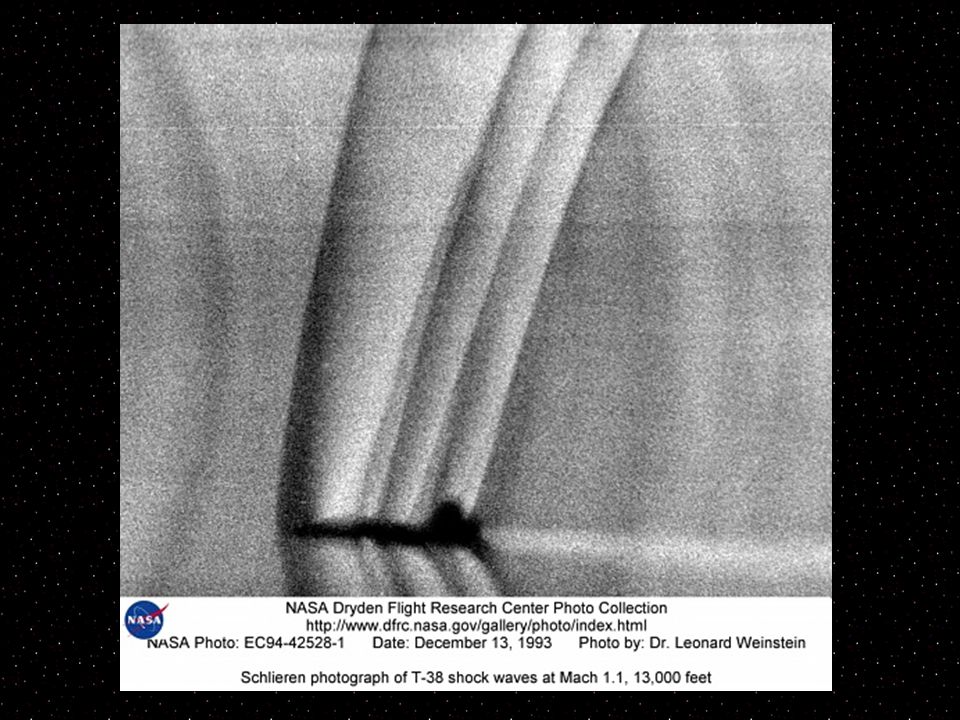
20. The Sound Barrier  A moving source of sound will produce wavefronts that are closer together than normal  The wavefronts get closer and closer together as the source moves faster and faster  At the speed of sound the wavefronts are all pushed together and form a shockwave called the Mach cone  In 1947 Chuck Yeager flew the X-1 faster than the speed of sound (~760 mph)  This is dangerous because passing through the shockwave makes the plane hard to control  In 1997 the Thrust SSC broke the sound barrier on land

21. Bell X-1

23. Thrust SSC