1. Chapter 7 Laplace Transforms

2. Applications of Laplace Transform notes Easier than solving differential equations –Used to describe system behavior –We assume LTI systems –Uses S-domain instead of frequency domain Applications of Laplace Transforms/ –Circuit analysis Easier than solving differential equations Provides the general solution to any arbitrary wave (not just LRC) –Transient –Sinusoidal steady-state-response (Phasors) –Signal processing –Communications Definitely useful for Interviews!

3. Building the Case… http://web.cecs.pdx.edu/~ece2xx/ECE222/Slides/LaplaceTransformx4.pdf

4. Laplace Transform

5. We use the following notations for Laplace Transform pairs – Refer to the table!

6. Laplace Transform Convergence The Laplace transform does not converge to a finite value for all signals and all values of s The values of s for which Laplace transform converges is called the Region Of Convergence (ROC) Always include ROC in your solution! Example: Remember: e^jw is sinusoidal; Thus, only the real part is important! 0+ indicates greater than zero values

7. Example of Bilateral Version Find F(s): Re(s)<a a S-plane Note that Laplace can also be found for periodic functions ROC Remember These!

8. Example – RCO may not always exist! Note that there is no common ROC  Laplace Transform can not be applied!

9. Example – Unilateral Version Find F(s):

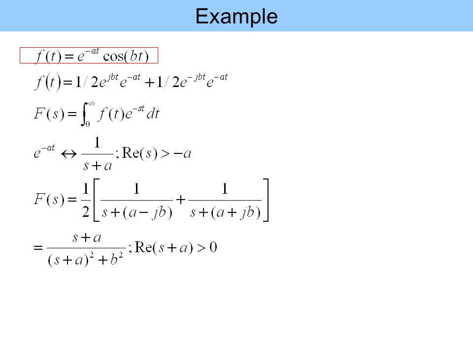
10. Example

12. Properties The Laplace Transform has many difference properties Refer to the table for these properties

13. Linearity

14. Scaling & Time Translation Scaling Time Translation b=0 Do the time translation first!

15. Shifting and Time Differentiation Shifting in s-domain Differentiation in t Read the rest of properties on your own!

16. Examples Note the ROC did not change!

17. Example – Application of Differentiation Read Section 7.4 Matlab Code: Read about Symbolic Mathematics: http://www.math.duke.edu/education/ccp/materials/diffeq/mlabtutor/mlabtut7.html And http://www.mathworks.de/access/helpdesk/help/toolbox/symbolic/ilaplace.html

18. Example What is Laplace of t^3? –From the table: 3!/s^4 Re(s)>0 Find the Laplace Transform: Note that without u(.) there will be no time translation and thus, the result will be different: Time transformation Assume t>0

19. A little about Polynomials Consider a polynomial function: A rational function is the ratio of two polynomials: A rational function can be expressed as partial fractions A rational function can be expressed using polynomials presented in product-of-sums Has roots and zeros; distinct roots, repeated roots, complex roots, etc. Given Laplace find f(t)!

20. Finding Partial Fraction Expansion Given a polynomial Find the POS (product-of-sums) for the denominator: Write the partial fraction expression for the polynomial Find the constants –If the rational polynomial has distinct poles then we can use the following to find the constants: http://cnx.org/content/m2111/latest/

21. Matlab Code Application of Laplace Consider an RL circuit with R=4, L=1/2. Find i(t) if v(t)=12u(t). Partial fraction expression Given

22. Application of Laplace What are the initial [i(0)] and final values: –Using initial-value property: –Using the final-value property Note: using Laplace Properties Note that Initial Value: t=0, then, i(t)  3-3=0 Final Value: t  INF then, i(t)  3

23. Using Simulink H(s) i(t) v(t )

24. Actual Experimentation Note how the voltage looks like: Input Voltage: Output Voltage:

25. Partial Fraction Expansion (no repeated Poles/Roots) – Example Using Matlab: Matlab code: b=[8 3 -21]; a=[1 0 -7 -6]; [r,p,k]=residue(b,a) We can also use ilaplace (F); but the result may not be simplified!

26. Finding Poles and Zeros Express the rational function as the ratio of two polynomials each represented by product-of-sums Example: S-plane Pole zero

27. H(s) Replacing the Impulse Response h(t) x(t)y(t) H(s) X(s)Y(s) convolution multiplication

28. H(s) Replacing the Impulse Response h(t) x(t)y(t) H(s) X(s)Y(s) convolution multiplication Example: Find the output X(t)=u(t); h(t) 0 1 1 h(t) 0 1 1 y(t) e^-sF(s) This is commonly used in D/A converters!

29. Dealing with Complex Poles Given a polynomial Find the POS (product-of-sums) for the denominator: Write the partial fraction expression for the polynomial Find the constants –The pole will have a real and imaginary part: P=|k|  When we have complex poles {|k|  then we can use the following expression to find the time domain expression: http://cnx.org/content/m2111/latest/

30. Laplace Transform Characteristics Assumptions: Linear Continuous Time Invariant Systems Causality –No future dependency –If unilateral: No value for t<0; h(t)=0 Stability –System mode: stable or unstable –We can tell by finding the system characteristic equation (denominator) Stable if all the poles are on the left plane –Bounded-input-bounded-output (BIBO) Invertability –H(s).Hi(s)=1 Frequency Response –H(w)=H(s);s  jw=H(s=jw) We need to add control mechanism to make the overall system stable

31. Frequency Response – Matlab Code

32. Inverse Laplace Transform

33. Example of Inverse Laplace Transform

34. Bilateral Transforms Laplace Transform of two different signals can be the same, however, their ROC can be different:  Very important to know the ROC. Signals can be –Right-sided  Use the bilateral Laplace Transform Table –Left-sides –Have finite duration How to find the transform of signals that are bilateral! See notes

35. How to Find Bilateral Transforms If right-sided use the table for unilateral Laplace Transform Given f(t) left-sided; find F(s): –Find the unilateral Laplace transform for f(-t)  laplace{f(-t)}; Re(s)>a –Then, find F(-s) with Re(-s)>a Given Fb(s) find f(t) left-sided : –Find the unilateral Inverse Laplace transform for F(s)=f b (t) –The result will be f(t)=–f b (t)u(-t) Example

36. Examples of Bilateral Laplace Transform Find the unilateral Laplace transform for f(-t)  laplace{f(-t)}; Re(s)>a Then find F(-s) with Re(-s)>a Alternatively: Find the unilateral Laplace transform for f(t)u(-t)  (-1)laplace{f(t)}; then, change the inequality for ROC.

37. Feedback System Find the system function for the following feedback system: G(s) Sum F(s) X(t) r(t) e(t)y(t) + + H(s) X(t)y(t) Equivalent System Feedback Applet: http://physioweb.uvm.edu/homeostasis/simple.htm

38. Practices Problems Schaum’s Outlines Chapter 3 –3.1, 3.3, 3.5, 3.6, 3.7-3.16,  For Quiz! –3.17-3.23 –Read section 7.8 –Read examples 7.15 and 7.16 Useful Applet: http://jhu.edu/signals/explore/index.html