1. Bounding Volume Hierarchy “Efficient Distance Computation Between Non-Convex Objects” Sean Quinlan Stanford, 1994 Presented by Mathieu Brédif

2. Simplifying Assumptions Surface analysis only Decomposition of objects into sets of convex surfaces Easy in graphics; all surfaces are composed of triangles Not necessarily easy in general

3. Basis: Convex Objects Efficient distance computation between convex polyhedra Decomposition of two objects into m and n convex polyhedra. O(mn) distance computation

4. Algorithm Overview Preprocessing: Approximation by Bounding Volume Hierarchies of Spheres Query: Branch and Bound in both trees to find minimum distance

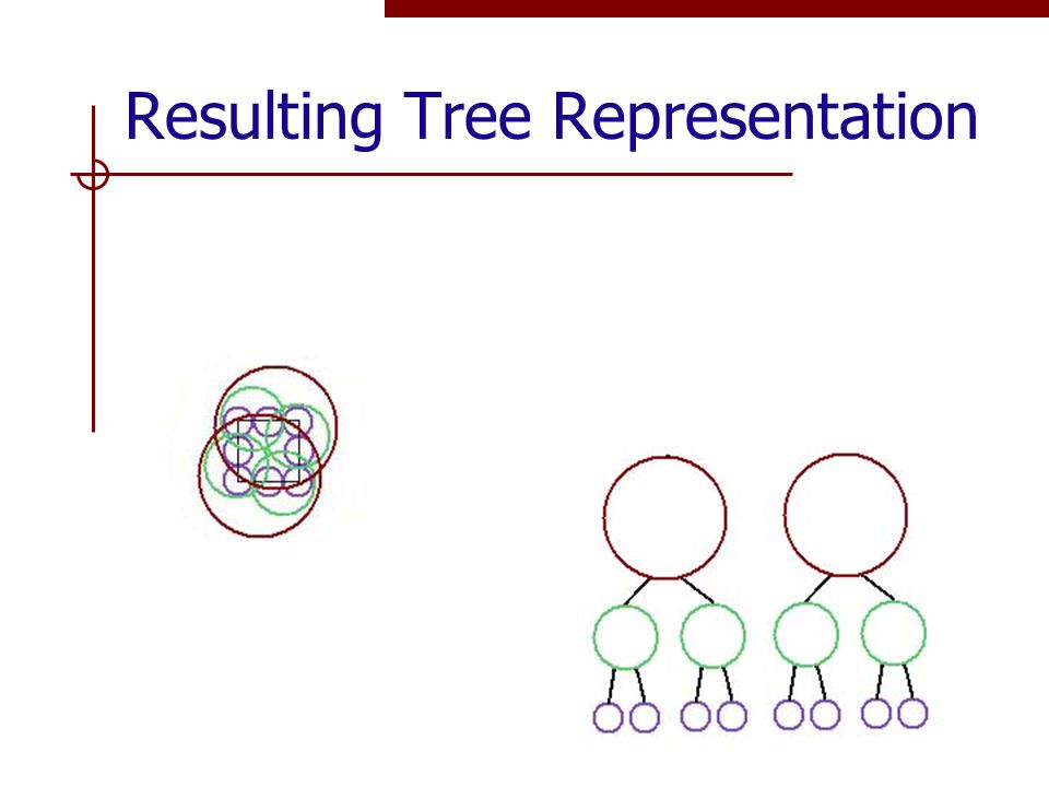
5. The Sphere Hierarchy Binary tree Root node = object’s bounding sphere Leaf nodes are tiny spheres; their union approximates the object’s surface Every node’s sphere contains entirely its descendents

6. Creating the Leaves Cover the object surface with tiny spheres (leaf nodes). Radius: user-determined.

7. Creating a ~balanced Tree Divide halfway in the major axis of a rectangular bounding box. Recurse until 1 leaf per set (Root down to leaves)

8. Decorating the Tree with Spheres Leaves up to root: create bounding spheres for each node. Best of 2 methods: Find the minimal sphere that contains the two spheres of the child nodes Determine a sphere directly from the leaf nodes descended from this node

9. Resulting Tree Representation

13. Query: Computing Distances Depth-first search on the binary tree Keep an updated minimum distance Depth-first  more pruning in search Prune search on branches that won’t reduce minimum distance Once leaf node is reached, examine underlying convex polygon for exact distance (former method)

14. Simple Example Set initial distance value to infinity Start at the root node. 20 < infinity, so continue searching

15. Simple Example Set initial distance value to infinity Start at the root node. 20 < infinity, so continue searching. 40 < infinity, so continue searching recursively. Choose the nearest of the two child spheres to search first

16. Simple Example Eventually search reaches a leaf node 40 < infinity; examine the polygon to which the leaf node is attached.

17. Simple Example Eventually search reaches a leaf node Call algorithm to find exact distance to the segment. Replace infinity with new minimum distance (42 in this case). 40 < infinity; examine the segment to which the leaf node is attached. d = 42

18. Simple Example Continue depth-first search 45 > 42; don’t search this branch any further

19. Simple Example Continue depth-first search 60 > 42; we can prune this half of our tree from the search 45 > 42; don’t search this branch any further

20. Efficiency: Building the Tree Roughly balanced binary tree Expected time O(n log n) Worst case time O(n 2 ) (n = #leaves nodes) Precomputed: Built only once!

21. Efficiency: Searching the Tree Full search O(n) to traverse the tree + O(p) time to compute distance to each polygon in the underlying model The algorithm allows a pruned search Worst case: no change! (close objects) Best case: O(log n) + a single polygon comparison

22. Collision Detection BVH: Two sphere trees 2 spheres intersects => descend further May need to descend to polygon level (line segment in 2D)

23. Collision Detection Quick Widely separated Collided Slower Close but not overlapping Close at many points

24. Extension: Multiple Trees If 2nd object is not a single point Start at root of both trees Branch: split the larger sphere The closest child to the unsplit sphere is searched first Deformable Object: precomputation of solid links, meta-tree computation before queries

25. Extension: Relative Error New minimum distance d Registration: d’ = (1-  )*d  user-determined relative error d’=0 iff d=0; correct collision detection Better pruning => performance speedup Exact distance in [d’,d’/(1-  )] Trade off: efficiency/exactitude

26. Empirical Results Relative error of 20% more pruning in search speedup of 2 orders of magnitude Objects close together less pruning in search less efficient

27. Conclusions Simple and intuitive way to speed up distance calculations Gives more information than collision detection algorithms Built on top of algorithms that compute distances between convex polygons Applications to path planning (robot=object1, obstacles=object2)