Infinite State Model Checking with Presburger Arithmetic Constraints Tevfik Bultan Department of Computer Science University of California, Santa Barbara.

Infinite State Model Checking with Presburger Arithmetic Constraints Tevfik Bultan Department of Computer Science University of California, Santa Barbara

Joint Work with My Students Action Language Verifier –Tuba Yavuz-Kahveci (PhD 2004) –Constantinos Bartzis (PhD 2004) Design for verification –Aysu Betin-Can (PhD 2005)

Infinite State Model Checking? Model checking started as a finite state verification technique Advantages of finite state systems: –Exhaustive state enumeration is possible for finite state systems Disadvantages of infinite state systems: –Verification problems that are computable for finite state systems are uncomputable for infinite state systems

Why Care About Infinity? Computer systems do not have infinite memory or infinite time –So why care about infinity? Infinity is an abstraction –Abstraction is at the core of computer science Computers are built with layers of abstractions –Abstraction is necessary for design –Abstraction is necessary for analysis

Why Care About Infinity? Reason 1: –Enables us to check a specification with respect to an arbitrarily large number of components or memory For example, arbitrary number of threads Reason 2: –Rather than developing verification techniques that rely on the bound of the state space to terminate Enables us to develop infinite state verification techniques that terminate independent of the bound A technique which is guaranteed to terminate is not helpful if it runs out of memory

An Example A simple example that demonstrates limitations of (finite state) model checkers Property P can be verified with an infinite state model checker that uses standard backward fixpoint computations Fixpoint computation for some properties  –for example, AG(State1  x  6) may not converge but we can use conservative approximations State0 State1 x’=x+1 x’=x+1 Initial: x=0  State0 P: AG(State1  x is odd) P: AG(State1  ( . x =2  +1))

Outline Model checking with arithmetic constraints Conservative approximations Automata representation for arithmetic constraints Composite representation Action Language Verifier (ALV) Checking synchronization in concurrent programs with ALV

Symbolic Model Checking [McMillan et al. LICS 1990] Represent sets of states and the transition relation as Boolean logic formulas Forward and backward fixpoints can be computed by iteratively manipulating these formulas –Forward, backward image: Existential variable elimination –Conjunction (intersection), disjunction (union) and negation (set difference), and equivalence check Use an efficient data structure for manipulation of Boolean logic formulas –BDDs

Symbolic Model Checking What do you need to compute fixpoints? Symbolic Conjunction(Symbolic,Symbolic) Symbolic Disjunction(Symbolic,Symbolic) Symbolic Negation(Symbolic) BooleanEquivalenceCheck(Symbolic,Symbolic) Symbolic Precondition(Symbolic) Precondition (i.e., EX) computation is handled by: –variable renaming, followed by conjunction, followed by existential variable elimination Infinite state model checking: Use a symbolic representation that is capable of representing infinite sets and supports the above functionality

Linear Arithmetic Constraints Linear arithmetic formulas can represent (infinite) sets of valuations of unbounded integers Linear integer arithmetic formulas on can be stored as a set of polyhedra is a linear equality or inequality constraint where each is a linear equality or inequality constraint and each is a polyhedron x i integer variable, a i coefficient, c constant

A Linear Arithmetic Constraint Manipulator Omega Library [Pugh et al.] –A tool for manipulating Presburger arithmetic formulas: First order theory of integers without multiplication –Equality and inequality constraints are not enough –Divisibility constraints are also needed which means: is divisible by

2y  x – 1 x – 5  2y 3y  x + 7 x  3y dark shadow real shadow 293 y x Integers are Complicated

Presburger Arithmetic Model Checking [Bultan et al. CAV’97, TOPLAS’99] Use linear arithmetic constraints as a symbolic representation Use a Presburger arithmetic manipulator as the symbolic engine (Omega library) Compute fixpoints to verify or falsify CTL properties Use conservative approximations to achieve convergence

What About Using BDDs for Encoding Arithmetic Constraints? Arithmetic constraints on bounded integer variables can be represented using BDDs Use a binary encoding –represent integer x as x 0 x 1 x 2... x k –where x 0, x 1, x 2,..., x k are binary variables –You have to be careful about the variable ordering! BDDs and constraint representations are both applicable –Which one is better?

Arithmetic Constraints vs. BDDs [Bultan TACAS’00]

Arithmetic Constraints vs. BDDs

Constraint based verification can be more efficient than BDDs for integers with large domains Constraint based verification can be used to automatically verify infinite state systems –cannot be done using BDDs However, BDD-based verification is more robust and the arithmetic constraint representation has two problems: Problem 1: Constraint based verification does not scale well when there are boolean or enumerated variables in the specification Problem 2: Price of infinity –CTL model checking becomes undecidable for infinite domains

Conservative Approximations Compute a lower ( p  ) or an upper ( p + ) approximation to the truth set of the property ( p )

Conservative Approximations Compute a lower ( p  ) or an upper ( p + ) approximation to the truth set of the property ( p ) There are three possible outcomes: I p pppp 1) “The property is satisfied”

Conservative Approximations Compute a lower ( p  ) or an upper ( p + ) approximation to the truth set of the property ( p ) There are three possible outcomes: I p pppp 1) “The property is satisfied” I p 3) “I don’t know” 2) “The property is false and here is a counter-example” I p  p p p p sates which violate the property p+p+p+p+ pppp

Conservative Approximations Truncated fixpoint computations –To compute a lower bound for a least-fixpoint computation –Stop after a fixed number of iterations Widening –To compute an upper bound for the least-fixpoint computation –We use a generalization of the polyhedra widening operator by [Cousot and Halbwachs POPL’78]

y  5 1  y x  4 x  y y x Polyhedra Widening A i : x  y  x  4  y  5  1  y

y  5 1  y x  4 x  y y x Polyhedra Widening x  y y  5 1  y x  5 A i : x  y  x  4  y  5  1  y A i+1 : x  y  x  5  y  5  1  y

y  5 1  y x  4 x  y y x Polyhedra Widening x  5 A i : x  y  x  4  y  5  1  y A i+1 : x  y  x  5  y  5  1  y A i  A i+1 : x  y  y  5  1  y

y  5 1  y x  4 x  y y x Polyhedra Widening x  y y  5 1  y x  5 A i : x  y  x  4  y  5  1  y A i+1 : x  y  x  5  y  5  1  y A i  A i+1 : x  y  y  5  1  y A i  A i+1 is defined as: all the constraints in A i that are also satisfied by A i+1

Automata Representation for Arithmetic Constraints [Bartzis, Bultan CIAA’02, IJFCS ’02] Given an atomic linear arithmetic constraint in one of the following two forms we can construct an FA which accepts all the solutions to the given constraint By combining such automata one can handle full Presburger arithmetic

Basic Construction We first construct a basic state machine which –Reads one bit of each variable at each step, starting from the least significant bits –and executes bitwise binary addition and stores the carry in each step in its state 012 0 1 0 / 0 1 01/101/1 1 / 0 1 0 / 0 1 1 / 1 11/011/0 00/100/1 Example x + 2y 010 + 2  001 100 01/001/0 1 0 / 0 Number of states: In my figures alphabet symbols are written vertically!

Automaton Construction Equality With 0 –All transitions writing 1 go to a sink state –State labeled 0 is the only accepting state –For disequations (  ), state labeled 0 is the only rejecting state Inequality (<0) –States with negative carries are accepting –No sink state Non-zero Constant Term c –Same as before, but now -c is the initial state –If there is no such state, create one (and possibly some intermediate states which can increase the size by |c|)

Conjunction and Disjunction 0 0 1 0,1,1 0 1 0,1 1010 1010 1010 0101 0 0 1 0,1,1 Automaton for x-y<1 0 1 0 0,1 0 1 0,1 0 1 1 1,0,1 1 0,1 0101 1010 Automaton for 2x-y>0 0 -2 1111 0101 1010 0000 0 0,1 1111 1010 1010 0101 0 1 0,1 0 1 1,1 1010 0000 0000 0 1 0,1 1010 0101 0 1 1,1 1010 Automaton for x-y 0 -1,-1 0,-1 -2,-1 -1,0 -2,0-2,1 Conjunction and disjunction is handled by generating the product automaton

Other Extensions Existential quantification (necessary for pre and post) –Project the quantified variables away –The resulting FA is non-deterministic Determinization may result in exponential blowup of the FA size but we do not observe this in practice –For universal quantification use negation Constraints on all integers –Use 2’s complement arithmetic –The basic construction is the same –In the worst case the size doubles

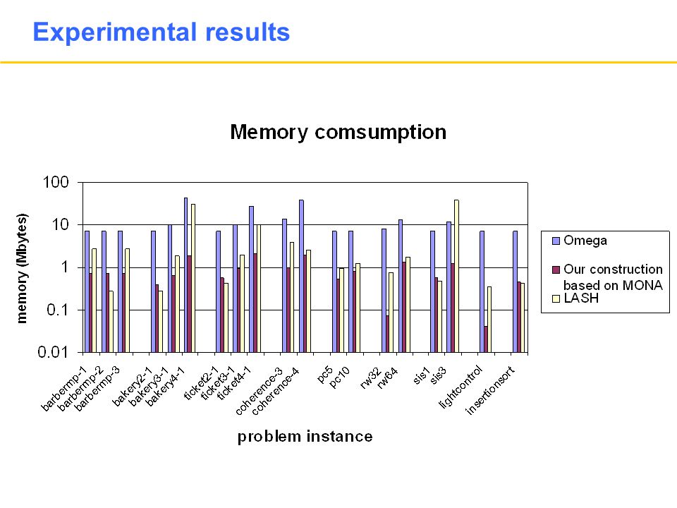
Experiments We implemented these algorithms using MONA [Klarlund et al] We integrated them to our infinite state model checker We compared our automata representation against –the polyhedral representation used in the Omega library –the automata representation used in LASH [Boigelot and Wolper] we also integrated LASH to our model checker by writing a wrapper around it

Experimental results

Efficient Pre- and Post-condition Computations [Bartzis, Bultan CAV’03] Pre and post condition computations can cause an exponential blow-up in the size of the automaton in the worst case We do not observe this blow-up in the experiments We proved that for a common class of systems this blow up does not occur

Assumptions About the Transition Relation We assume that the transition relation of the input system is a disjunction of formulas in the following form guard(R)  update(R) where –guard(R) is a Presburger formula on current state variables and –update(R) is of the form x i ’=f(x 1, …, x v )   x j ’= x j In asynchronous concurrent systems the transition relation is usually in the above form jiji

Three Classes of Updates 1.x i ’ = c 2.x i ’ = x i + c 3.x i ’ =  j=1 a j · x j + c We proved that Computation of pre is polynomial for all 3 cases Computation of post is polynomial for 2 and for 3, whenever a i is odd. v

Other Results Related to Automata Encoding [Bartzis, Bultan TACAS’03, STTT] We developed efficient BDD construction algorithms and proved bounds for the sizes of the BDDs for bounded linear arithmetic constraints –Given a linear arithmetic formula that contains n atomic constraints on v bounded integer variables represented with b-bits, the size of the BDD is: These results explain why all three versions of SMV (NuSMV, CMU SMV and Cadence SMV) are inefficient in handling linear arithmetic constraints –In SMV the BDD size could be exponential in b

Other Results Related to Automata Encoding [CAV’04] We defined a widening operator for the automata representation of arithmetic constraints The widening operator looks for similar states in two consecutive iterations (A i and A i+1 ) and creates an equivalence relation –then it merges the states in the same equivalence class We can prove that for some cases this widening operator computes the exact fixpoint –for example for updates of the form x’=x+c

Example The sequence y=x, y=x  y=x+1, y=x  y=x+1  y=x+2, … does not converge However we know that a fixpoint exists (y  x) and is representable as an arithmetic constraint module incr_1 integer y; parameterized integer x; initial: y=x; incr_1: y'=y+1; spec: AG(y>=x) endmodule

Widening Instead of computing a sequence A 1, A 2, … where A i+1 =A i  post(A i ) compute A’ 1, A’ 2, … where A’ i+1 =A’ i  (A’ i  post(A’ i )) By definition A  B  A  B The goal is to find a widening operator  such that: –The sequence A’ 1, A’ 2, … converges –It converges fast –The computed fixpoint is as close as possible to the exact set of reachable states

Widening Arithmetic Automata Given automata A and A’ we want to compute A  A’ We say that states k and k’ are equivalent (k  k’) if either –k and k’ can be reached from either initial state with the same string (unless k or k’ is a sink state) –or, the languages accepted from k and k’ are equal –or, for some state k’’, k  k’’ and k’  k’’ The states of A  A’ are the equivalence classes of 

Example 0 1 0,1 1 0 0,1 XXXX 01 y=x 0 X 0,1 0 1 2 3 0 1 0,1 0 1 0,1 1 0 0,1 1010 1010 0101 XXXX y=x  y=x+1 0 1 0 1 2 3 01 3

Example 0 1 0,1 1 0 0,1 XXXX 01 0 X 0,1 0 1 2 3 0 1 0,1 0 1 0,1 1 0 0,1 1010 1010 0101 XXXX = 0 X 0,1 1010 1010 2 0101 3 XXXX 0 1 0,1

Example 0 0, 1010 1 0 01 0101 2 X X 0 1 0,1 X0X0 0 0000 0 X 0,1 2 1 1010 34 X X X 1 1 0 0101 1010 0101 0 1 0,1 1 0 0 1 2 0 1 2 3 4 1 0 2 3 4 X 1

Example X0X0 0 0000 0 X 0,1 2 1 1010 34 XXXX X1X1 1010 0101 1010 0101 0 1 0,1 1010 0 0, 1010 1010 01 0101 2 XXXX 0 1 0,1 X1X1 0 X 0,1 1010 X 1 0,0 0,21,3 0101 = Represents: y  x

Composite Model Checking [Bultan, Gerber, League ISSTA 98, TOSEM 00] Map each variable type to a symbolic representation –Map boolean and enumerated types to BDD representation –Map integer type to a linear arithmetic constraint representation Use a disjunctive representation to combine different symbolic representations: composite representation Each disjunct is a conjunction of formulas represented by different symbolic representations –we call each disjunct a composite atom

Composite Representation symbolic rep. 1 symbolic rep. 2 symbolic rep. t composite atom Example: x: integer, y: boolean x>0 and x´  x-1 and y´ or x<=0 and x´  x and y´  y arithmetic constraint representation BDD arithmetic constraint representation BDD

Composite Symbolic Library [Yavuz-Kahveci, Tuncer, Bultan TACAS01], [Yavuz-Kahveci, Bultan FroCos 02, STTT 03] Uses a common interface for each symbolic representation Easy to extend with new symbolic representations Enables polymorphic verification Multiple symbolic representations: –As a BDD library we use Colorado University Decision Diagram Package (CUDD) [Somenzi et al] –As an integer constraint manipulator we use Omega Library [Pugh et al]

Composite Symbolic Library Class Diagram CUDD LibraryOMEGA Library Symbolic +intersect() +union() +complement() +isSatisfiable() +isSubset() +pre() +post() CompSym –representation: list of comAtom +intersect() + union() BoolSym –representation: BDD +intersect() +union() IntSym –representation: Polyhedra +intersect() +union() compAtom –atom: *Symbolic

Pre and Post-condition Computation Variables: x: integer, y: boolean Transition relation: R: x>0 and x´  x-1 and y´ or x<=0 and x´  x and y´  y Set of states: s: x=2 and !y or x=0 and !y Compute post(s,R)

Pre and Post-condition Distribute R: x>0 and x´  x-1 and y´ or x<=0 and x´  x and y´  y s: x=2 and !y or x=0 and y post(s,R) = post( x=2, x>0 and x´  x-1 )  post( !y, y´ ) x=1 y  post( x=2, x<=0 and x´  x )  post ( !y, y´  y ) false !y  post( x=0, x>0 and x´  x-1 )  post( y, y´ ) false y  post ( x=0, x<=0 and x´  x )  post ( y, y´  y ) x=0 y = x=1 and y or x=0 and y

Polymorphic Verifier Symbolic TranSys::check(Node *f) { Symbolic s = check(f.left) case EX: s.pre(transRelation) case EF: do sold = s s.pre(transRelation) s.union(sold) while not sold.isEqual(s) }  Action Language Verifier is polymorphic  It becomes a BDD based model checker when there or no integer variables

Composite Representation + Shape Graphs [Yavuz-Kahveci, Bultan SAS 02] Shape graphs represent the states of the heap Each node in the shape graph represents a dynamically allocated memory location Heap variables point to nodes of the shape graph The edges between the nodes show the locations pointed by the fields of the nodes add top next next n1n2 heap variables add and top point to node n1 add.next is node n2 top.next is also node n2 add.next.next is null

Composite Symbolic Library: Further Extended CUDD LibraryOMEGA Library Symbolic +union() +isSatisfiable() +isSubset() +forwardImage() CompSym –representation: list of comAtom + union() BoolSym –representation: BDD +union() compAtom –atom: *Symbolic HeapSym –representation: list of ShapeGraph +union() IntSym –representation: list of Polyhedra +union() ShapeGraph –atom: *Symbolic

Forward Fixpoint pc=l1  mutex numItems=2 add top   pc=l2   mutex  numItems=2 addtopBDD arithmetic constraint representation A set of shape graphs  pc=l4   mutex  numItems=2  addtop  pc=l1  mutex  numItems=3  addtop

Post-condition Computation: Example pc=l4   mutex  numItems=2  addtop pc=l4 and mutex’ pc’=l1 pc=l1  mutex numItems’=numItems+1  numItems=3 top’=add   addtop set of states transitionrelation

Again: Fixpoints Do Not Converge We have two reasons for non-termination –integer variables can increase without a bound –the number of nodes in the shape graphs can increase without a bound As I mentioned earlier, we use widening on integer variables to achieve convergence For heap variables we use the summarization operation

Summarization Example pc=l1  mutex numItems=3 add top   pc=l1  mutex numItems=3  summarycount=2 add top  summary node a new integer variable representing the number of concrete nodes encoded by the summary node After summarization, it becomes: summarized nodes

Simplification pc=l1  mutex  numItems=3  summaryCount=2 addtop pc=l1  mutex add top   numItems=4  summaryCount=3  = pc=l1  mutex add top   (numItems=4  summaryCount=3  numItems=3  summarycount=2)

Simplification On the Integer Part pc=l1  mutex add top   (numItems=4  summaryCount=3  numItems=3  summaryCount=2) = pc=l1  mutex add top  numItems=summaryCount+1  3  numItems  numItems  4

Then We Use Integer Widening pc=l1  mutex add top  numItems=summaryCount+1  3  numItems  numItems  4 pc=l1  mutex add top  numItems=summaryCount+1  3  numItems  numItems  5  pc=l1  mutex add top  numItems=summaryCount+1  3  numItems = Now, fixpoint converges

Verified Properties SpecificationVerified Invariants Stack top=null  numItems=0 top  null  numItems  0 numItems=2  top.next  null Single Lock Queue head=null  numItems=0 head  null  numItems  0 (head=tail  head  null)  numItems=1 head  tail  numItems  0 Two Lock Queue numItems>1  head  tail numItems>2  head.next  tail

Verifying Linked Lists with Multiple Fields Pattern-based summarization –User provides a graph grammar rule to describe the summarization pattern L x = next x y, prev y x, L y Represent any maximal sub-graph that matches the pattern with a summary node –no node in the sub-graph pointed by a heap variable

Summarization Pattern Examples... nnn L x  x.n = y, L y... nnn L x  x.n = y, y.p = x, L y ppp L x  x.n = y, x.d = z, L y... nnn d d d

Action Language Tool Set Action Language Parser Verifier (ALV) OmegaLibraryCUDDPackage MONA Composite Symbolic Library PresburgerArithmeticManipulatorBDDManipulatorAutomataManipulator Action Language Specification Verified Counter example

Action Language [Bultan, ICSE 00], [Bultan, Yavuz-Kahveci, ASE 01] Variables: boolean, enumerated, integer (unbounded) Parameterized constants –specifications are verified for all possible values Transition relation is defined using actions and modules –Atomic actions: Predicates on current and next state variables –Action composition: asynchronous (|) or synchronous (&) –A module is defined as asynchronous and/or synchronous compositions of its actions and submodules

Readers Writers Example: A Closer Look module main() integer nr; boolean busy; restrict: nr>=0; initial: nr=0 and !busy; module Reader() boolean reading; initial: !reading; rEnter: !reading and !busy and nr’=nr+1 and reading’; rExit: reading and !reading’ and nr’=nr-1; Reader: rEnter | rExit; endmodule module Writer()... endmodule main: Reader() | Reader() | Writer() | Writer(); spec: invariant(busy => nr=0) endmodule S : Cartesian product of variable domains defines variable domains defines the set of states the set of states I : Predicates defining the initial states the initial states R : Atomic actions of the Reader Reader R : Transition relation of Reader defined as asynchronous composition of its atomic actions R : Transition relation of main defined as asynchronous composition of two Reader and two Writer processes

Arbitrary Number of Threads Counting abstraction –Create an integer variable for each local state of a thread –Each variable will count the number of threads in a particular state Local states of the threads have to be finite –Specify only the thread behavior that relates to the correctness of the controller –Shared variables of the controller can be unbounded Counting abstraction can be automated

Readers-Writers After Counting Abstraction module main() integer nr; boolean busy; parameterized integer numReader, numWriter; restrict: nr>=0 and numReader>=0 and numWriter>=0; initial: nr=0 and !busy; module Reader() integer readingF, readingT; initial: readingF=numReader and readingT=0; rEnter: readingF>0 and !busy and nr’=nr+1 and readingF’=readingF-1 and readingT’=readingT+1; rExit: readingT>0 and nr’=nr-1 readingT’=readingT-1 and readingF’=readingF+1; Reader: rEnter | rExit; endmodule module Writer()... endmodule main: Reader() | Writer(); spec: invariant(busy => nr=0) endmodule Variables introduced by the counting abstractions Parameterized constants introduced by the counting abstractions

Verification of Readers-Writers IntegersBooleansCons. Time (secs.) Ver. Time (secs.) Memory (Mbytes) RW-4150.040.016.6 RW-8190.080.017 RW-161170.190.028 RW-321330.530.0310.8 RW-641651.710.0620.6 RW-P710.050.019.1

Design for Verification Action Language Verifier Verification of Synchronization in Concurrent Programs Design for Verification uses enables

A Java Read-Write Lock Implementation class ReadWriteLock { private Object lockObj; private int totalReadLocksGiven; private boolean writeLockIssued; private int threadsWaitingForWriteLock; public ReadWriteLock() { lockObj = new Object(); writeLockIssued = false; } public void getReadLock() { synchronized (lockObj) { while ((writeLockIssued) || (threadsWaitingForWriteLock != 0)) { try { lockObj.wait(); } catch (InterruptedException e) { } } totalReadLocksGiven++; } } public void getWriteLock() { synchronized (lockObj) { threadsWaitingForWriteLock++; while ((totalReadLocksGiven != 0) || (writeLockIssued)) { try { lockObj.wait(); } catch (InterruptedException e) { // } } threadsWaitingForWriteLock--; writeLockIssued = true; } } public void done() { synchronized (lockObj) { //check for errors if ((totalReadLocksGiven == 0) && (!writeLockIssued)) { System.out.println(" Error: Invalid call to release the lock"); return; } if (writeLockIssued) writeLockIssued = false; else totalReadLocksGiven--; lockObj.notifyAll(); } } } How do we translate this to Action Language? Action Language Verifier Verification of Synchronization in Java Programs

Design for Verification Abstraction and modularity are key both for successful designs and scalable verification techniques The question is: –How can modularity and abstraction at the design level be better integrated with the verification techniques which depend on these principles? Our approach: –Structure software in ways that facilitate verification –Document the design decisions that can be useful for verification –Improve the applicability and scalability of verification using this information

A Design for Verification Approach We have been investigating a design for verification approach based on the following principles: 1.Use of design patterns that facilitate automated verification 2.Use of stateful, behavioral interfaces which isolate the behavior and enable modular verification 3.An assume-guarantee style modular verification strategy that separates verification of the behavior from the verification of the conformance to the interface specifications 4.A general model checking technique for interface verification 5.Domain specific and specialized verification techniques for behavior verification Avoids usage of error-prone Java synchronization primitives: synchronize, wait, notify Separates controller behavior from the threads that use the controller: Supports a modular verification approach which exploits this modularity for scalable verification

class Action{ protected final Object owner; … private boolean GuardedExecute(){ boolean result=false; for(int i=0; i<gcV.size(); i++) try{ if(((GuardedCommand)gcV.get(i)).guard()){ ((GuardedCommand)gcV.get(i)).update(); result=true; break; } }catch(Exception e){} return result; } public void blocking(){ synchronized(owner) { while(!GuardedExecute()) { try{owner.wait();} catch (Exception e){} } owner.notifyAll(); } } public boolean nonblocking(){ synchronized(owner) { boolean result=GuardedExecute(); if (result) owner.notifyAll(); return result; } } class RWController implements RWInterface{ int nR; boolean busy; final Action act_r_enter, act_r_exit; final Action act_w_enter, act_w_exit; RWController() {... gcs = new Vector(); gcs.add(new GuardedCommand() { public boolean guard(){ return (nR == 0 && !busy);} public void update(){busy = true;}} ); act_w_enter = new Action(this,gcs); } public void w_enter(){ act_w_enter.blocking();} public boolean w_exit(){ return act_w_exit.nonblocking();} public void r_enter(){ act_r_enter.blocking();} public boolean r_exit(){ return act_r_exit.nonblocking();} } Reader-Writer Controller This helper class is provided. No need to rewrite it!

Controller Interfaces A controller interface defines the acceptable call sequences for the threads that use the controller Interfaces are specified using finite state machines public class RWStateMachine implements RWInterface{ StateTable stateTable; final static int idle=0,reading=1, writing=2; public RWStateMachine(){... stateTable.insert("w_enter",idle,writing); } public void w_enter(){ stateTable.transition("w_enter"); }... } writing reading idle r_enter r_exit w_exit w_enter

Concurrent Program Controller Classes Thread Classes Controller Interface Machine Controller Behavior Machine Java Path Finder Action Language Verifier Thread Isolation Thread Class Counting Abstraction Interface Verification Behavior Verification Verification Framework

Interface Machine Thread 1Thread 2Thread n Thread 1 Controller Shared Data Interface Machine Thread 2 Interface Machine Thread n Thread Modular Interface Verification Concurrent Program Controller Behavior Modular Behavior Verification Modular Design / Modular Verification Interface

Behavior Verification Analyzing properties (specified in CTL) of the synchronization policy encapsulated with a concurrency controller and its interface –Verify the controller properties assuming that the user threads adhere to the controller interface Behavior verification with Action Language Verifier –We wrote a translator which translates controller classes to Action Language –Using counting abstraction we can check concurrency controller classes for arbitrary number of threads

Interface Verification A thread is correct with respect to an interface if all the call sequences generated by the thread can also be generated by the interface machine –Checks if all the threads invoke controller methods in the order specified in the interfaces –Checks if the threads access shared data only at the correct interface states Interface verification with Java PathFinder –Verify Java implementations of threads –Correctness criteria are specified as assertions Look for assertion violations Assertions are in the StateMachine and SharedStub –Performance improvement with thread Isolation

Thread Isolation: Part 1 Interaction among threads Threads can interact with each other in only two ways: –invoking controller actions –invoking shared data methods To isolate the threads –Replace concurrency controllers with controller interface state machines –Replace shared data with shared stubs

Thread Isolation: Part 2 Interaction among a thread and its environment Modeling thread’s call to its environment with stubs –File I/O, updating GUI components, socket operations, RMI call to another program Replace with pre-written or generated stubs Modeling the environment’s influence on threads with drivers –Thread initialization, RMI events, GUI events Enclose with drivers that generate all possible events that influence controller access

Automated Airspace Concept Automated Airspace Concept by NASA researchers automates the decision making in air traffic control The most important challenge is achieving high dependability Automated Airspace Concept includes a failsafe short term conflict detection component called Tactical Separation Assisted Flight Environment (TSAFE) –It is responsible for detecting conflicts in flight plans of the aircraft within 1 minute from the current time –Dependability of this component is even more important than the dependability of the rest of the system –It should be a smaller, isolated component compared to the rest of the system so that it can be verified

TSAFE TSAFE functionality: 1.Display aircraft position 2.Display aircraft planned route 3.Display aircraft future projected route trajectory 4.Show conformance problems

Server Computation Flight Database Graphical Client > 21,057 lines of code with 87 classes Radar feed > User EventThread Feed Parser Timer TSAFE Architecture

Behavior Verification Performance RW0.171.03 Mutex0.010.23 Barrier0.010.64 BB-RW0.136.76 BB-Mutex0.631.99 ControllerTime(sec)Memory (MB)P-Time (sec)P-Memory (MB) 8.1012.05 0.980.03 0.010.50 0.6310.80 2.056.47 P denotes parameterized verification for arbitrary number of threads

Interface Verification Performance ThreadTime (sec)Memory (MB) TServer-Main67.7217.08 TServer-RMI91.7920.31 TServer-Event6.5710.95 TServer-Feed123.1283.49 TClient-Main2.002.32 TClient-RMI17.0640.96 TClient-Event663.2133.09

Fault Categories Concurrency controller faults –initialization faults (2) –guard faults (2) –update faults (6) –blocking/nonblocking faults (4) Interface faults –modified-call faults (8) –conditional-call faults conditions based on existing program variables (13) conditions on new variables declared during fault seeding (5)

Effectiveness in Finding Faults Created 40 faulty versions of TSAFE Each version had at most one interface fault and at most one behavior fault –14 behavior and 26 interface faults Among 14 behavior faults ALV identified 12 of them –2 uncaught faults were spurious Among 26 interface faults JPF identified 21 of them –2 of the uncaught faults were spurious –3 of the uncaught faults were real faults that were not caught by JPF

Falsification Performance TServer-RMI29.4324.74 TServer-Event6.889.56 TServer-Feed18.5194.72 TClient-RMI10.1242.64 TClient-Event15.6312.20 ThreadTime (sec)Memory (MB) RW-80.343.26 RW-161.6110.04 RW-P1.515.03 Mutex-80.020.19 Mutex-160.040.54 Mutex-p0.120.70 Concurrency ControllerTime (sec)Memory (MB)

Conclusions Infinite state model checking is feasible –Enables verification of specifications with unbounded variables –Enables verification of parameterized systems Infinite state verification techniques can help us in identifying more efficient finite state model checking techniques Building extensible tools is important!

Conclusions Application of automated verification techniques to real- world systems leads to re-thinking the design –Design for verification can lead to more effective verification Integrating verification tools lead to more effective verification –In our case ALV and JPF

Conclusions We were able to use our design for verification approach based on design patterns and behavioral interfaces in different domains Use of domain specific behavior verification techniques has been very effective –Interface verification was the bottleneck Model checking research resulted in various verification techniques and tools which can be customized for specific classes of software systems Automated verification techniques can scale to realistic software systems using design for verification approach

THE END

Infinite State Model Checking with Presburger Arithmetic Constraints Tevfik Bultan Department of Computer Science University of California, Santa Barbara.

Similar presentations

Presentation on theme: "Infinite State Model Checking with Presburger Arithmetic Constraints Tevfik Bultan Department of Computer Science University of California, Santa Barbara."— Presentation transcript:

Similar presentations

About project

Feedback

Log in

Auth with social network:

Infinite State Model Checking with Presburger Arithmetic Constraints Tevfik Bultan Department of Computer Science University of California, Santa Barbara.

Similar presentations

Presentation on theme: "Infinite State Model Checking with Presburger Arithmetic Constraints Tevfik Bultan Department of Computer Science University of California, Santa Barbara."— Presentation transcript:

Similar presentations

About project

Feedback