1. Electromagnetic Induction
Chapter 21
Electromagnetic Induction
Faraday’s Law
ac Circuits
We found in chapter 20 that an electric current can give rise to a magnetic field, and that a magnetic field can exert a force on a moving charge.
I wonder if a magnetic field can somehow give rise to an electric current…

2. 21.1 Induced emf
It is observed experimentally that changes in magnetic fields induce an emf in a conductor.
An electric current is induced if there is a closed circuit (e.g., loop of wire) in the changing magnetic field.
A constant magnetic field does not induce an emf—it takes a changing magnetic field.
Passing the coil through the magnet would induce an emf in the coil.
They need to calibrate their meter!

3. Note that “change” does not require observable (to you) motion.
 A magnet may move through a loop of wire, or a loop of wire may be moved through a magnetic field (as suggested in the previous slide). These involve observable motion.
 A changing current in a loop of wire gives rise to a changing magnetic field (predicted by Ampere’s law) which can induce a current in another nearby loop of wire.
In the latter case, nothing observable (to your eye) is moving, although, of course microscopically, electrons are in motion.
As your text puts it: “induced emf is produced by a changing magnetic field.”

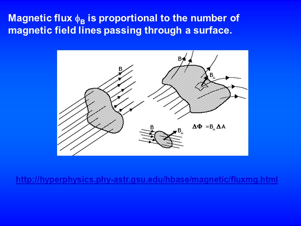
4. 21.2 Faraday’s Law
To quantify the ideas of section 21.1, we define magnetic flux. In an earlier chapter we briefly touched on electric flux. This is the magnetic analog.
Because we can’t “see” magnetic fields directly, we draw magnetic field lines to help us visualize the magnetic field. Remember that magnetic field lines start at N poles and end at S poles.
A strong magnetic field is represented by many magnetic field lines, close together. A weak magnetic field is represented by few magnetic field lines, far apart.
We could, if we wished, actually “calibrate” by specifying the number of magnetic field lines passing through some surface that corresponded to a given magnetic field strength.

5. Magnetic flux B is proportional to the number of magnetic field lines passing through a surface.

6. Mathematically, magnetic flux B through a surface of area A is defined by
B = B A cos 
OSE: B = BA
where B is the component of field perpendicular to the surface, A is the area of the surface, and  is the angle between B and the normal to the surface. B A 
B B A

7. 
B
B=0 A
When B is parallel to the surface, =90° and B = 0.
=0
B=0 B A
When B is perpendicular to the surface, =0° and B = BA.
The unit of magnetic flux is the Tm2, called a weber:
1 Wb = 1 T  m2 .

8. In the following discussion, we switch from talking about surfaces in a magnetic field…
…to talking about loops of wire in a magnetic field.

9. Now we can quantify the induced emf described qualitatively in the previous section
Experimentally, if the flux through N loops of wire changes by an amount B in a time t, the induced emf is
Not an OSE—not quite yet.
This is called Faraday’s law of induction. It is one of the fundamental laws of electricity and magnetism, and an important component of the theory that explains electricity and magnetism.
I wonder why the – sign…

10. Among other things, conservation of energy would be violated.
Experimentally…
…an induced emf always gives rise to a current whose magnetic field opposes the change in flux—Lenz’s law.*
Think of the current resulting from the induced emf as “trying” to maintain the status quo—to prevent change.
If Lenz’s law were not true—if there were a + sign in faraday’s law—then a changing magnetic field would produce a current, which would further increased the magnetic field, further increasing the current, making the magnetic field still bigger…
Among other things, conservation of energy would be violated.
*We’ll practice with this in a bit.

11. Ways to induce an emf:
 change B
 change the area of the loop in the field

12. Ways to induce an emf (continued):
 change the orientation of the loop in the field

13. Conceptual example 21-1 Induction Stove
An ac current in a coil in the stove top produces a changing magnetic field at the bottom of a metal pan.
The changing magnetic field gives rise to a current in the bottom of the pan.
Because the pan has resistance, the current heats the pan. If the coil in the stove has low resistance it doesn’t get hot but the pan does.
An insulator won’t heat up on an induction stove.
Remember the controversy about cancer from power lines a few years back? Careful studies showed no harmful effect. Nevertheless, some believe induction stoves are hazardous.

14. Conceptual example 21-2 Practice with Lenz’s Law
In which direction is the current induced in the coil for each situation shown?
(counterclockwise)
(no current)

15. (counterclockwise)
(clockwise)

16. Rotating the coil about the vertical diameter by pulling the left side toward the reader and pushing the right side away from the reader in a magnetic field that points from right to left in the plane of the page.
(counterclockwise)
Remember
Now that we are experts on the application of Lenz’s law, lets make our induced emf equation official:
This means it is up to you to use Lenz’s law to figure out the direction of the induced current (or the direction of whatever the problem wants.

17. Example 21-3 Pulling a Coil from a Magnetic Field
A square coil of side 5 cm contains 100 loops and is positioned perpendicular to a uniform 0.6 T magnetic field. It is quickly and uniformly pulled from the field (moving  to B) to a region where the field drops abruptly to zero. It takes 0.10 s to remove the coil, whose resistance is 100 . 
B = 0.6 T
5 cm

18. (a) Find the change in flux through the coil.
Initial: Bi = BA .
Final: Bf = 0 .
B = Bf - Bi = 0 - BA = - (0.6 T) (0.05 m)2 = - 1.5x10-3 Wb .

19. (b) Find the current and emf induced. 
The current must flow counterclockwise to induce a downward magnetic field (which replaces the “removed” magnetic field).

20. The induced emf is
The induced current is

21. (c) How much energy is dissipated in the coil?
Current flows “only*” during the time flux changes.
E = Pt = I2Rt = (1.5x10-2 A) (100 ) (0.1 s) = 2.3x10-3 J .
(d) What was the average force required?
The loop had to be “pulled” out of the magnetic field, so the pulling force did work. It is tempting to try and set up a free body diagram and use Newton’s laws. Instead, energy conservation gets the answer with less work.
*If there no resistance in the loop, the current would flow indefinitely. However, the resistance quickly halts the flow of current once the magnetic flux stops changing.

22. The flux change occurs only when the coil is in the process of leaving the region of magnetic field.
No flux change.
No emf.
No current.
No work (why?).

23. Flux changes. emf induced. Current flows. Work done. F D
Flux changes. emf induced. Current flows. Work done.

24. No flux change. No emf. No current. (No work.)
No flux change. No emf. No current. (No work.)

25. The energy calculated in part (c) is the energy dissipated in the coils while the current is flowing. The amount calculated in part (c) is also the mechanical energy put into the system by the force.
Ef – Ei = [ Wother]If
See 2 slides back for F and D.
Ef – Ei = F D
F = Ef / D
F = (2.3x10-3 J) / (0.05 m)
F = N

26. 21.3 emf Induced in a Moving Conductor
Recall that one of the ways to induce an emf is to change the area of the loop in the magnetic field. Let’s see how this works. v B 
A U-shaped conductor and a moveable conducting rod are placed in a magnetic field, as shown. ℓ
The rod moves to the right with a speed v for a time t. A
vt
The rod moves a distance vt and the area of the loop inside the magnetic field increases by an amount
A = ℓ v t .

27. The loop is perpendicular to the magnetic field, so the magnetic flux through the loop is B = BA. The emf induced in the conductor can be calculated using Ampere’s law:
B and v are vector magnitudes, so they are always +. Wire length is always +. You use Lenz’s law to get the direction of the current.

28. This “kind” of emf is called “motional emf” because it took motion to induce it.
The induced emf causes current to flow in the loop. v B 
Magnetic flux inside the loop increases (more area). ℓ
System “wants” to make the flux stay the same, so the current gives rise to a field inside the loop into the plane of the paper (to counteract the “extra” flux). I A
vt
Clockwise current!

29. The induced emf causes current to flow in the loop
The induced emf causes current to flow in the loop. Giancoli shows an alternate method for getting , by calculating the work done moving the charges in the wire. v ℓ B 
vt A I
Electrons in the moving rod (only the rod moves) experience a force F = q v B. Using the right hand rule,* you find the the force is “up” the rod, so electrons move “up.”
“Up” here refers only to the orientation on the page, and has nothing to do with gravity.
Because the rod is part of a loop, electrons flow counterclockwise, and the current is clockwise (whew, we got that part right!).
*Remember, find the force direction, then reverse it if the charge is an electron!

30. The work to move an electron from the bottom of the rod to the top of the rod is W = (force) (distance) = (q v B) (ℓ).
Going way back to the beginning of the semester, Wif = q Vif .
F = q v B v ℓ B 
vt A I
But Vif is just the change in potential along the length ℓ of the loop, which is the induced emf.
Going way back to the beginning of the semester, W = (q v B) (ℓ) = (q ).
Solving (q v B) (ℓ) = (q ) for  gives  = B ℓ v, as before.

31. I won’t ask you to reproduce the derivation on an exam, but a problem could (intentionally or not) ask you to calculate the work done in moving a charge (or a wire) through a magnetic field, so be sure to study your text.
“But you haven’t given us the OSE yet!”
Good point! The derivation assumed B, ℓ, and v are all mutually perpendicular, so we really derived this:
where B is the component of the magnetic field perpendicular to ℓ and v, and v is the component of the velocity perpendicular to B and ℓ.

32. Example An airplane travels 1000 km/h in a region where the earth’s field is 5x10-5 T and is nearly vertical. What is the potential difference induced between the wing tips that are 70 m apart?  v
The derivation of  = B ℓ v on slides 15 and 16 assumed the area through which the magnetic field passes increased.
My first reaction is that the magnetic flux through the wing is not changing because neither the field nor the area of the wing is changing.
True, but wrong reaction! The alternate derivation shows that the electrons in the moving rod (airplane wing in this case) experience a force, which moves the electrons.

33. The electrons “pile up” on the left hand wing of the plane, leaving an excess of + charge on the right hand wing.  v - +
Our equation for  gives the potential difference.
No danger to passengers! (But I would want my airplane designers to be aware of this.)

34. 21.4 Changing Magnetic Flux Produces an Electric Field
From chapter 16, section 6:
OSE: E = F / q
From chapter 20, section 4:
OSE: F = q v B sin
For v  B, and in magnitude only,
F = q E = q v B
E = v B.
We conclude that a changing magnetic flux produces an electric field. This is true not just in conductors, but any-where in space where there is a changing magnetic field.

35. Example Blood contains charged ions, so blood flow can be measured by applying a magnetic field and measuring the induced emf. If a blood vessel is 2 mm in diameter and a 0.08 T magnetic field causes an induced emf of 0.1 mv, what is the flow velocity of the blood?
OSE:  = B ℓ v
v =  / (B ℓ)
In Figure (the figure for this example), B is applied  to the blood vessel, so B is  to v. The ions flow along the blood vessel, but the emf is induced across the blood vessel, so ℓ is the diameter of the blood vessel.
v = (0.1x10-3 V) / (0.08 T 0.2x10-3 m)
v = 0.63 m/s

36. 21.5 Electric Generators
Let’s begin by looking at a simple animation of a generator.
Here’s a “freeze-frame.”
Normally, many coils of wire are wrapped around an armature. The picture shows only one.
Brushes pressed against a slip ring make continual contact.
The shaft on which the armature is mounted is turned by some mechanical means.

37. Let’s look at the current direction in this particular freeze-frame.
B is down. Coil rotates counter-clockwise.
Put your fingers along the direction of movement. Stick out your thumb.
Bend your fingers 90°. Rotate your hand until the fingers point in the direction of B. Your thumb points in the direction of conventional current.

38. Alternative right-hand rule for current direction.
B is down. Coil rotates counter-clockwise.
Make an xyz axes out of your thumb and first two fingers.
Thumb along component of wire velocity  to B. 1st finger along B.
2nd finger then points in direction of conventional current.
Hey! The picture got it right!

39. I know we need to work on that more. Let’s zoom in on the armature.v
vB
vB I B

40. Forces on the charges in these parts of the wire are perpendicular to the length of the wire, so they don’t contribute to the net current.
For future use, call the length of wire shown in green “h” and the other lengths (where the two red arrows are) “ℓ”.

41. One more thing…
This wire…
…connects to this ring…
…so the current flows this way.

42. Later in the cycle, the current still flows clockwise in the loop…
…but now this wire…
…connects to this ring…
…so the current flows this way.
Alternating current! ac!
Again:

43. “Dang. That was complicated
“Dang! That was complicated. Are you going to ask me to do that on the exam?”
No. Not anything that complicated. But you still need to understand each step, because each step is test material.
Click here and scroll down to “electrodynamics” to see some visualizations that might help you!
Understanding how a generator works is “good,” but we need to quantify our knowledge.
We begin with our OSE  = B ℓ v. (ℓ was defined on slide 16.) In our sample generator on the last 7 slides, we had only one loop, but two sides of the loop in the magnetic field. If the generator has N loops, then  = 2 N B ℓ v.

44. Back to this picture: v
vB
vB B I
This picture is oriented differently than Figure in your text. In your text,  is the angle between the perpendicular to the magnetic field and the plane of the loop.

45.  v
vB
vB B I
The angle  is the text is the same as the angle between vB and the vector v.
Thus, v = v sin .

46. B is  to the wire, so
But the coil is rotating, so  =  t, and v =  r =  (h/2). The diameter of the circle of rotation, h, was defined on slide 16.
where A is the area of the loop, f is the frequency of rotation of the loop, and  = 2  f.

47. Example 21-6 The armature of a 60 Hz ac generator rotates in a 0
Example The armature of a 60 Hz ac generator rotates in a 0.15 T magnetic field. If the area of the coil is 2x10-2 m2, how many loops must the coil contain if the peak output is to be 0 = 170 V?

48. 18-8 Alternating Current
In chapter 21 we learned how a coil of wire rotating in a magnetic field creates ac current.
A large magnet rotating inside coils of wire would also produce ac current. (ac current is redundant, isn’t it?)

49. The voltage produced by the generator is sinusoidal:
The generator web page uses U instead of V as the symbol for voltage.

50. In chapter 21, we wrote
Using  = 2f, V instead of , and grouping constants together, in chapter 18 Giancoli “decrees” the formula
V0 is the “peak voltage” and in the US, the frequency of ac power in your home is f = 60 Hz.
Using Ohm’s law:
Where I0 is the peak current.

51. Note that the equations for Pavg contain
Even though the average current is zero, power is still lost due to resistance:
It is easy to show (a bit of calculus) that the average value of sin2(2 f t) is ½, so the average power developed in a resistance is
The bar above the P denotes “average.” I will write it Pavg when using text.
Note that the equations for Pavg contain
sorry, eqn. editor won’t let me put bar over 2 characters

52. The rms (root mean square) value of a quantity is obtained by taking the square root of the average of the square of that quantity. The equations for Pavg contain the mean square values of current and voltage.
We write
and
Then
Not sure why I didn’t make this “official” last year. I think I’ll make it “official” this year…

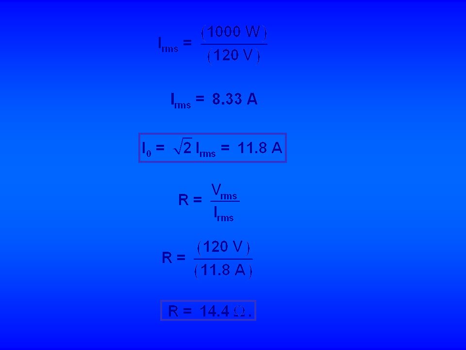
53. Un the US, we talk about rms voltage when we refer to household line voltage. The peak voltage is thus
Example (a) Calculate the resistance and the peak current in a 1000 W hair dryer connected to a 120 V line. (b) what happens if it is connected to a 240 V line in Britain?
(a) Our OSE P = IV = I2R = V2/R works if we replace P by Pavg and I and V by Irms and Vrms.

55. (b) Assume the hair dryer’s resistance does not change with temperature (in reality, it probably increases).
You just melted your hair dryer!

56. Example Each channel of a stereo receiver is capable of an average power output of 100 W into an 8  loudspeaker. What is the rms voltage and rms current fed to the speaker (a) at the maximum power of 100 W, and (b) at 1 W?
we’ll use these for both parts

57. (a) at 100 W and 8 :
(b) at 1 W and 8 :

58. 21-7 Transformers

59. No, no, no…
A transformer is a device for increasing or decreasing an ac voltage.
Pole-mounted transformer
ac-dc converter
Power Substation

60. A transformer is basically two coils of wire wrapped around each other, or wrapped around an iron core.
When an ac voltage is applied to the primary coil, it induces an ac voltage in the secondary coil.
A “step up” transformer increases the output voltage in the secondary coil; a “step down” transformer reduces it.

61. The ac voltage in the primary coil causes a magnetic flux change given by
The changing flux (which is efficiently “carried” in the transformer core) induces an ac voltage in the secondary coil given by
Dividing the two equations gives the transformer equation
For a step-up transformer, NS > NP and VS > VP (the voltage is stepped up).

62. For a step-down transformer, NS < NP and VS < VP (the voltage is stepped down).
Transformers only work with ac voltages; a dc voltage does not produce the necessary changing flux.
A step-up transformer increases the voltage. Is this an example of “getting something for nothing?”
No, because even though transformers are extremely efficient, some power (and therefore energy) is lost.
If no power is lost, we can use P = IV to get
flipped!

63. If transformers only work on ac, how come you showed a picture of an ac-dc converter a few slides back?
Ever wanted to cut open one of those ac-dc converters and see what they look like inside?
An ac-dc converter first steps down the 120 volt line voltage, and then converts the voltage to dc:
fewer turns in the secondary coil
a diode is a device that lets current flow one way only (dc)

64. Pictures of ac-dc converter came from http://www. howstuffworks
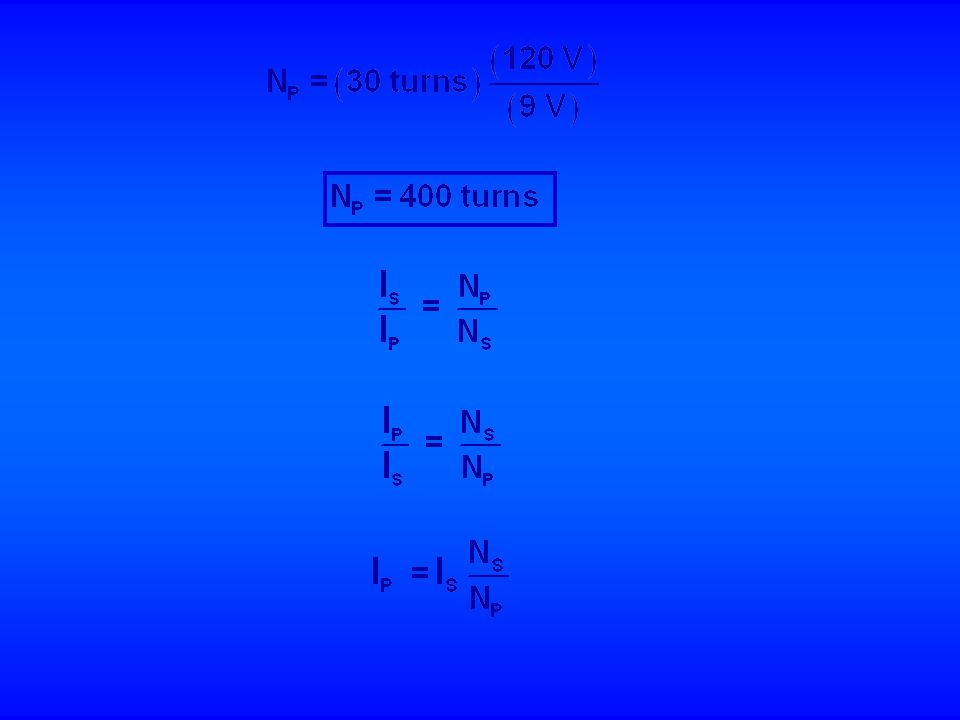
Example 21-9 A transformer for home use of a portable radio reduces 120 V ac to 9 V dc. The secondary contains 30 turns and the radio draws 400 mA. Calculate (a) the number of turns in the primary; (b) the current in the primary; and (c) the power transformed.

66. The power output to the secondary coil is
This is the same as the power input to the primary coil because our transformer equation derivation assumed 100% efficient transformation of power.

67. Example An average of 120 kW of electrical power is sent to a small town from a power plant 10 km away. The transmission lines have a total resistance of 0.40 . Calculate the power loss if power is transmitted at (a) 240 V and (b) 24,000 V.
This problem does not use the transformer equation, but it shows why transformers are useful.

68. (a) at 240 V
(a) at V
More than 80% of the power would be wasted if it were transmitted at 240 V, but less than 0.01 % is wasted if the power is transmitted at V.

69.
We skipped section 21.6 on counter emf. Read it to see why motors burn out when they can’t turn, and why your house lights might dim when the fridge comes on.

70. Electromagnetic Waves
Chapter 22
Electromagnetic Waves
Every student of E&M should be “exposed” to electromagnetic waves. Here is your exposure.
22.1 Maxwell’s Equations
Maxwell’s equations involve calculus. They represent the fundamental laws of electricity and magnetism. We have seen simpler forms of some of them.

71. In words, Maxwell’s equations are:
1—a generalized form of Coulomb’s law, relating electric fields to their sources (charges)
2—a law relating magnetic fields to magnetic poles
3—an equation describing how an electric field is produced by a changing magnetic field (Faraday’s Law)
4—an equation describing how a magnetic field is produced by an electric current or changing electric field (Ampere’s Law)
That a changing electric field can produce a magnetic field is not one of the predictions of Ampere’s law; it was hypothesized by Maxwell and verified after his death.

72. Every student should be exposed to Maxwell’s equations, so here they are in their integral form…

73. Electromagnetic Waves
Maxwell’s equations are to E&M as Newton’s laws are to mechanics, except Maxwell’s equations are relativistically correct, and Newton’s laws are not.
22.3 Production of
Electromagnetic Waves
Your text shows how electromagnetic waves can be produced by oscillating charges on conductors.
These waves travel through space even long after they are far away from the charges that produced them.
E and B in the radiation fields drop off as 1/r, and the intensity of the waves drops off as 1/r2.

74. The electric and magnetic fields are perpendicular to each other and to the direction of propagation of the wave. They are also in phase. See figure 22.7, page 666.
From Maxwell’s equations you can show that electromagnetic waves travel with a speed v = 1/(00)1/2 which is equal to 3x108 m/s, the speed of light.

75. The Electromagnetic Spectrum
22.5 Light as an E&M Wave
The Electromagnetic Spectrum
Light was known to behave like a wave long before Maxwell showed that the speed of E&M waves is the same as the speed of light. Eventually, it came to be recognized that light is just an example of an E&M wave.
The frequencies of visible light lie between about 4x10-7 and 7.5x10-7 m, or 400 to 750 nm. The frequency, wavelength, and speed of a wave are related by v = f, so for E&M waves, and for light, c = f.
Visible light represents only a minute portion of the electromagnetic spectrum, see figure E&M waves are typically produced by acceleration of charged particles.

76. The sun emits large amounts of IR, visible, and UV radiation
The sun emits large amounts of IR, visible, and UV radiation. We detect the IR as heat, the visible as light, and the UV through skin damage. Note from figure that x-rays, gamma rays, and radio waves are “just” E&M waves, like light, only of different frequencies.
(sorry, rushed scan)

77. Symbols for cut and paste
   ℓ  °            