1. Hadoop Technical Workshop Module III: MapReduce Algorithms

2. Algorithms for MapReduce Sorting Searching Indexing Classification Joining TF-IDF PageRank Clustering

3. MapReduce Jobs Tend to be very short, code-wise –IdentityReducer is very common “Utility” jobs can be composed Represent a data flow, more so than a procedure

4. Sort: Inputs A set of files, one value per line. Mapper key is file name, line number Mapper value is the contents of the line

5. Sort Algorithm Takes advantage of reducer properties: (key, value) pairs are processed in order by key; reducers are themselves ordered Mapper: Identity function for value (k, v)  (v, _) Reducer: Identity function (k’, _) -> (k’, “”)

6. Sort: The Trick (key, value) pairs from mappers are sent to a particular reducer based on hash(key) Must pick the hash function for your data such that k 1 hash(k 1 ) < hash(k 2 )

7. Final Thoughts on Sort Used as a test of Hadoop’s raw speed Essentially “IO drag race” Highlights utility of GFS

8. Search: Inputs A set of files containing lines of text A search pattern to find Mapper key is file name, line number Mapper value is the contents of the line Search pattern sent as special parameter

9. Search Algorithm Mapper: –Given (filename, some text) and “pattern”, if “text” matches “pattern” output (filename, _) Reducer: –Identity function

10. Search: An Optimization Once a file is found to be interesting, we only need to mark it that way once Use Combiner function to fold redundant (filename, _) pairs into a single one –Reduces network I/O

11. Indexing: Inputs A set of files containing lines of text Mapper key is file name, line number Mapper value is the contents of the line

12. Inverted Index Algorithm Mapper: For each word in (file, words), map to (word, file) Reducer: Identity function

13. Index: MapReduce map(pageName, pageText): foreach word w in pageText: emitIntermediate(w, pageName); done reduce(word, values): foreach pageName in values: AddToOutputList(pageName); done emitFinal(FormattedPageListForWord);

14. Index: Data Flow

15. An Aside: Word Count Word count was described in module I Mapper for Word Count is (word, 1) for each word in input line –Strikingly similar to inverted index –Common theme: reuse/modify existing mappers

16. Bayesian Classification Files containing classification instances are sent to mappers Map (filename, instance)  (instance, class) Identity Reducer

17. Bayesian Classification Existing toolsets exist to perform Bayes classification on instance –E.g., WEKA, already in Java! Another example of discarding input key

18. Joining Common problem: Have two data types, one includes references to elements of the other; would like to incorporate data by value, not by reference Solution: MapReduce Join Pass

19. Join Mapper Read in all values of joiner, joinee classes Emit to reducer based on primary key of joinee (i.e., the reference in the joiner, or the joinee’s identity)

20. Join Reducer Joinee objects are emitted as-is Joiner objects have additional fields populated by Joinee which comes to the same reducer as them. –Must do a secondary sort in the reducer to read the joinee before emitting any objects which join on to it

21. TF-IDF Term Frequency – Inverse Document Frequency –Relevant to text processing –Common web analysis algorithm

22. The Algorithm, Formally | D | : total number of documents in the corpus : number of documents where the term t i appears (that is ).

23. Information We Need Number of times term X appears in a given document Number of terms in each document Number of documents X appears in Total number of documents

24. Job 1: Word Frequency in Doc Mapper –Input: (docname, contents) –Output: ((word, docname), 1) Reducer –Sums counts for word in document –Outputs ((word, docname), n) Combiner is same as Reducer

25. Job 2: Word Counts For Docs Mapper –Input: ((word, docname), n) –Output: (docname, (word, n)) Reducer –Sums frequency of individual n’s in same doc –Feeds original data through –Outputs ((word, docname), (n, N))

26. Job 3: Word Frequency In Corpus Mapper –Input: ((word, docname), (n, N)) –Output: (word, (docname, n, N, 1)) Reducer –Sums counts for word in corpus –Outputs ((word, docname), (n, N, m))

27. Job 4: Calculate TF-IDF Mapper –Input: ((word, docname), (n, N, m)) –Assume D is known (or, easy MR to find it) –Output ((word, docname), TF*IDF) Reducer –Just the identity function

28. Working At Scale Buffering (doc, n, N) counts while summing 1’s into m may not fit in memory –How many documents does the word “the” occur in? Possible solutions –Ignore very-high-frequency words –Write out intermediate data to a file –Use another MR pass

29. Final Thoughts on TF-IDF Several small jobs add up to full algorithm Lots of code reuse possible –Stock classes exist for aggregation, identity Jobs 3 and 4 can really be done at once in same reducer, saving a write/read cycle Very easy to handle medium-large scale, but must take care to ensure flat memory usage for largest scale

30. PageRank: Random Walks Over The Web If a user starts at a random web page and surfs by clicking links and randomly entering new URLs, what is the probability that s/he will arrive at a given page? The PageRank of a page captures this notion –More “popular” or “worthwhile” pages get a higher rank

31. PageRank: Visually

32. PageRank: Formula Given page A, and pages T 1 through T n linking to A, PageRank is defined as: PR(A) = (1-d) + d (PR(T 1 )/C(T 1 ) +... + PR(T n )/C(T n )) C(P) is the cardinality (out-degree) of page P d is the damping (“random URL”) factor

33. PageRank: Intuition Calculation is iterative: PR i+1 is based on PR i Each page distributes its PR i to all pages it links to. Linkees add up their awarded rank fragments to find their PR i+1 d is a tunable parameter (usually = 0.85) encapsulating the “random jump factor” PR(A) = (1-d) + d (PR(T 1 )/C(T 1 ) +... + PR(T n )/C(T n ))

34. Graph Representations The most straightforward representation of graphs uses references from each node to its neighbors

35. Direct References Structure is inherent to object Iteration requires linked list “threaded through” graph Requires common view of shared memory (synchronization!) Not easily serializable class GraphNode { Object data; Vector out_edges; GraphNode iter_next; }

36. Adjacency Matrices Another classic graph representation. M[i][j]= '1' implies a link from node i to j. Naturally encapsulates iteration over nodes 01014 00103 11012 10101 4321

37. Adjacency Matrices: Sparse Representation Adjacency matrix for most large graphs (e.g., the web) will be overwhelmingly full of zeros. Each row of the graph is absurdly long Sparse matrices only include non-zero elements

38. Sparse Matrix Representation 1: (3, 1), (18, 1), (200, 1) 2: (6, 1), (12, 1), (80, 1), (400, 1) 3: (1, 1), (14, 1) …

39. Sparse Matrix Representation 1: 3, 18, 200 2: 6, 12, 80, 400 3: 1, 14 …

40. PageRank: First Implementation Create two tables 'current' and 'next' holding the PageRank for each page. Seed 'current' with initial PR values Iterate over all pages in the graph, distributing PR from 'current' into 'next' of linkees current := next; next := fresh_table(); Go back to iteration step or end if converged

41. Distribution of the Algorithm Key insights allowing parallelization: –The 'next' table depends on 'current', but not on any other rows of 'next' –Individual rows of the adjacency matrix can be processed in parallel –Sparse matrix rows are relatively small

42. Distribution of the Algorithm Consequences of insights: –We can map each row of 'current' to a list of PageRank “fragments” to assign to linkees –These fragments can be reduced into a single PageRank value for a page by summing –Graph representation can be even more compact; since each element is simply 0 or 1, only transmit column numbers where it's 1

44. Phase 1: Parse HTML Map task takes (URL, page content) pairs and maps them to (URL, (PR init, list-of-urls)) –PR init is the “seed” PageRank for URL –list-of-urls contains all pages pointed to by URL Reduce task is just the identity function

45. Phase 2: PageRank Distribution Map task takes (URL, (cur_rank, url_list)) –For each u in url_list, emit (u, cur_rank/|url_list|) –Emit (URL, url_list) to carry the points-to list along through iterations PR(A) = (1-d) + d (PR(T 1 )/C(T 1 ) +... + PR(T n )/C(T n ))

46. Phase 2: PageRank Distribution Reduce task gets (URL, url_list) and many (URL, val) values –Sum vals and fix up with d –Emit (URL, (new_rank, url_list)) PR(A) = (1-d) + d (PR(T 1 )/C(T 1 ) +... + PR(T n )/C(T n ))

47. Finishing up... A subsequent component determines whether convergence has been achieved (Fixed number of iterations? Comparison of key values?) If so, write out the PageRank lists - done! Otherwise, feed output of Phase 2 into another Phase 2 iteration

48. PageRank Conclusions MapReduce runs the “heavy lifting” in iterated computation Key element in parallelization is independent PageRank computations in a given step Parallelization requires thinking about minimum data partitions to transmit (e.g., compact representations of graph rows) –Even the implementation shown today doesn't actually scale to the whole Internet; but it works for intermediate-sized graphs

49. Clustering What is clustering?

50. Google News They didn’t pick all 3,400,217 related articles by hand… Or Amazon.com Or Netflix…

51. Other less glamorous things... Hospital Records Scientific Imaging –Related genes, related stars, related sequences Market Research –Segmenting markets, product positioning Social Network Analysis Data mining Image segmentation…

52. The Distance Measure How the similarity of two elements in a set is determined, e.g. –Euclidean Distance –Manhattan Distance –Inner Product Space –Maximum Norm –Or any metric you define over the space…

53. Hierarchical Clustering vs. Partitional Clustering Types of Algorithms

54. Hierarchical Clustering Builds or breaks up a hierarchy of clusters.

55. Partitional Clustering Partitions set into all clusters simultaneously.

56. Partitional Clustering Partitions set into all clusters simultaneously.

57. K-Means Clustering Simple Partitional Clustering Choose the number of clusters, k Choose k points to be cluster centers Then…

58. K-Means Clustering iterate { Compute distance from all points to all k- centers Assign each point to the nearest k-center Compute the average of all points assigned to all specific k-centers Replace the k-centers with the new averages }

59. But! The complexity is pretty high: –k * n * O ( distance metric ) * num (iterations) Moreover, it can be necessary to send tons of data to each Mapper Node. Depending on your bandwidth and memory available, this could be impossible.

60. Furthermore There are three big ways a data set can be large: –There are a large number of elements in the set. –Each element can have many features. –There can be many clusters to discover Conclusion – Clustering can be huge, even when you distribute it.

61. Canopy Clustering Preliminary step to help parallelize computation. Clusters data into overlapping Canopies using super cheap distance metric. Efficient Accurate

62. Canopy Clustering While there are unmarked points { pick a point which is not strongly marked call it a canopy center mark all points within some threshold of it as in it’s canopy strongly mark all points within some stronger threshold }

63. After the canopy clustering… Resume hierarchical or partitional clustering as usual. Treat objects in separate clusters as being at infinite distances.

64. MapReduce Implementation: Problem – Efficiently partition a large data set (say… movies with user ratings!) into a fixed number of clusters using Canopy Clustering, K-Means Clustering, and a Euclidean distance measure.

65. The Distance Metric The Canopy Metric ($) The K-Means Metric ($$$)

66. Steps! Get Data into a form you can use (MR) Picking Canopy Centers (MR) Assign Data Points to Canopies (MR) Pick K-Means Cluster Centers K-Means algorithm (MR) –Iterate!

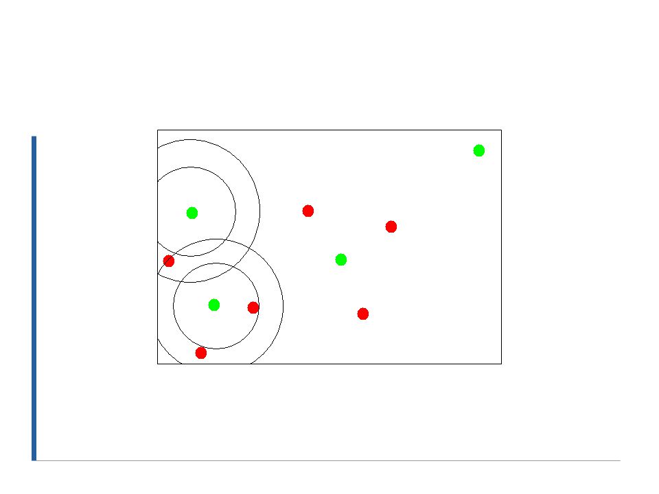
67. Selecting Canopy Centers

83. Assigning Points to Canopies

89. K-Means Map

97. Elbow Criterion Choose a number of clusters s.t. adding a cluster doesn’t add interesting information. Rule of thumb to determine what number of Clusters should be chosen. Initial assignment of cluster seeds has bearing on final model performance. Often required to run clustering several times to get maximal performance

98. Clustering Conclusions Clustering is slick And it can be done super efficiently And in lots of different ways

99. Conclusions Lots of high level algorithms Lots of deep connections to low-level systems

100. Aaron Kimball aaron@cloudera.com