Download presentation
Presentation is loading. Please wait.

1
Matrix A matrix is a rectangular array of elements arranged in rows and columns Dimension of a matrix is r x c r = c square matrix r = 1 (row) vector c = 1 column vector
 vector c = 1 column vector")
2
Matrix (cont) elements are either numbers or symbols each element is designated by the row and column that it is in, a ij rows are indicated by an i subscript columns are indicated by a j subscript
 elements are either numbers or symbols each element is designated by the row and column that it is in, a ij rows are indicated by an i subscript columns are indicated by a j subscript")
3
Matrix Equality two matrices are said to be equal if they have the same dimensions and all of the corresponding elements are equal

4
Equality: Example Are the following matrices equal? a) b)
 b)")
5
Matrix Operations - Transpose A transposition is performed by switching the rows and columns, indicated by a ‘ A’ = B if a ij = b ji Note: if A is r x c then B will be c x r The transpose of a column vector is a row vector.

6
Matrix Operations – Addition/Subtraction To add or subtract two matrices, they must have the same dimensions The addition or subtraction is done on an element by element bases

7
Matrix Operations - Multiplication by a scalar (number) every element of the matrix is multiplied by that number In addition, a matrix can be factored if A = [a ij ], k is a number then kA = Ak = [ka ij ]
![Matrix Operations - Multiplication by a scalar (number) every element of the matrix is multiplied by that number In addition, a matrix can be factored if A = [a ij ], k is a number then kA = Ak = [ka ij ]](http://images.slideplayer.com/16/4913066/slides/slide_7.jpg "Matrix Operations - Multiplication by a scalar (number) every element of the matrix is multiplied by that number In addition, a matrix can be factored if A = [a ij ], k is a number then kA = Ak = [ka ij ]")
8
Matrix Operations - Multiplication by another matrix – C = A B columns of A must equal rows of B Resulting matrix has dimension rows of A x columns of B

9
Special Types of Matrices: Symmetric if A = A’, then A is said to be symmetric a symmetric matrix has to be a square matrix

10
Special Types of Matrices: Diagonal Square matrix with off-diagonal elements equal to 0.

11
Special Types of Matrices: Diagonal (cont) Identity also called the unit matrix, designated by I a diagonal matrix where the diagonal elements are 1 It is called the identity matrix because for any matrix A AI = IA = A
 Identity also called the unit matrix, designated by I a diagonal matrix where the diagonal elements are 1 It is called the identity matrix because for any matrix A AI = IA = A")
12
Linear Dependence Think of the columns of a matrix as column vectors if it can be found that not all of k 1 to k c are 0 in the following equation then the c columns are linearly dependent. k 1 C 1 + k 2 C 2 + + k c C c = 0 In the example -2C 1 + 0C 2 + 1C 3 = 0 if they all 0, then they are linearly independent.

13
Rank of a Matrix The rank of a matrix is the maximum number of linearly independent columns. This is a unique number for every matrix rank of the matrix cannot exceed min(r,c) Full Rank – all columns are linearly independent Example: Rank = 2
 Full Rank – all columns are linearly independent Example: Rank = 2.")
14
Inverse of a Matrix Inverse in algebra: – reciprocal – Inverse for a matrix – A A -1 = A -1 A = I – A must be square and full rank

15
Inverse of a Matrix: Calculation Diagonal Matrix

16
Inverse of a Matrix: Calculation (cont) 2 x 2 Matrix 1.Calculate the Determinant: D = ad – bc If D = 0, then the matrix doesn’t have full rank (singular) and does not have an inverse. 2.A -1 : switch a and d, make b and c negative, divide by D. 3 x 3 Matrix: in the book

17
Inverse of a Matrix: Uses In algebra, we use the inverse to solve algebraic equations. In matrix algebra, we use the inverse of a matrix to solve matrix algebraic equations: A X = C A -1 A X = A -1 C X = A -1 C

18
Basic Matrix Operations A + B = B + A (A + B) + C = A + (B + C) k(A + B) = k A + kB (A’)’ = A (A + B)’ = A’ + B’ (AB)’ = B’ A’ (ABC)’ = C’B’ A’ (AB)C = A(BC) C(A + B) = C A + CB (A -1 ) -1 = A (A’) -1 = (A -1 )’ (AB) -1 = B -1 A -1 (ABC) -1 = C -1 B -1 A -1
 + C = A + (B + C) k(A + B) = k A + kB (A’)’ = A (A + B)’ = A’ + B’ (AB)’ = B’ A’ (ABC)’ = C’B’ A’ (AB)C = A(BC) C(A + B) = C A + CB (A -1 ) -1 = A (A’) -1 = (A -1 )’ (AB) -1 = B -1 A -1 (ABC) -1 = C -1 B -1 A -1")
19
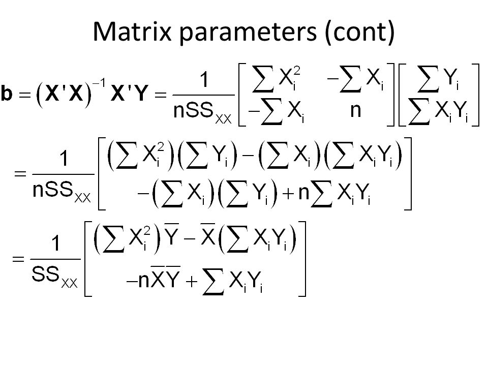
Matrix parameters

20
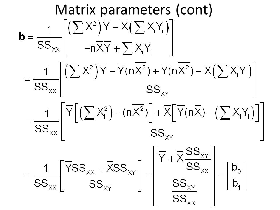
Matrix parameters (cont)
")
23
Fitted Values

24
Response Vector: additive (Surface.sas) Ŷ i = -2.79 + 2.14 X i,1 + 1.21 X i,2
 Ŷ i = X i, X i,2")
25
SAS code: MLR proc reg data = a1; model y = x1 x2 x3; run;

26
Response Vector: polynomial (Surface.sas) Ŷ i = 150+ 2.14 X i,1 – 4.02 X 2 i,1 + 1.21 X i,2 + 10.14 X 2 i,2
 Ŷ i = X i,1 – 4.02 X 2 i, X i, X 2 i,2")
27
Response Vector: Interaction(Surface.sas) Ŷ i = 10.5 + 3.21 X i,1 + 1.2 X i,2 – 1.24 X i,1 X i,2
 Ŷ i = X i, X i,2 – 1.24 X i,1 X i,2")
28
SAS code: MLR data a2; set a1; xsq = x*x; x12 = x1*x2; proc reg data=a2; model y = x xsq x1 x2 x12; run;

29
CS Example: all predictors (output ) Analysis of Variance SourceDFSum of Squares Mean Square F ValuePr > F Model528.643645.7287311.69<.0001 Error218106.819140.49000 Corrected Total223135.46279 Root MSE0.70000R-Square0.2115 Dependent Mean2.63522Adj R-Sq0.1934 Coeff Var26.56311 Parameter Estimates VariableDFParameter Estimate Standard Error t ValuePr > |t| Intercept10.326720.400000.820.4149 hsm10.145960.039263.720.0003 hss10.035910.037800.950.3432 hse10.055290.039571.400.1637 satm10.000943590.000685661.380.1702 satv1-0.000407850.00059189-0.690.4915
 Analysis of Variance SourceDFSum of Squares Mean Square F ValuePr > F Model <.0001 Error Corrected Total Root MSE R-Square Dependent Mean Adj R-Sq Coeff Var Parameter Estimates VariableDFParameter Estimate Standard Error t ValuePr > |t| Intercept hsm hss hse satm satv")
30
ANOVA table for MLR SourcedfSSMSFp Model (Regression) p – 1Σ(Ŷ i - Y̅) 2 p Errorn – pΣ(Y i - Ŷ i ) 2 Totaln - 1Σ(Y i - Y̅) 2
 p – 1Σ(Ŷ i - Y̅) 2 p Errorn – pΣ(Y i - Ŷ i ) 2 Totaln - 1Σ(Y i - Y̅) 2")
31
CS Example: all predictors (output ) Analysis of Variance SourceDFSum of Squares Mean Square F ValuePr > F Model528.643645.7287311.69<.0001 Error218106.819140.49000 Corrected Total223135.46279 Root MSE0.70000R-Square0.2115 Dependent Mean2.63522Adj R-Sq0.1934 Coeff Var26.56311 Parameter Estimates VariableDFParameter Estimate Standard Error t ValuePr > |t| Intercept10.326720.400000.820.4149 hsm10.145960.039263.720.0003 hss10.035910.037800.950.3432 hse10.055290.039571.400.1637 satm10.000943590.000685661.380.1702 satv1-0.000407850.00059189-0.690.4915
 Analysis of Variance SourceDFSum of Squares Mean Square F ValuePr > F Model <.0001 Error Corrected Total Root MSE R-Square Dependent Mean Adj R-Sq Coeff Var Parameter Estimates VariableDFParameter Estimate Standard Error t ValuePr > |t| Intercept hsm hss hse satm satv")
32
CS Example: (cs.sas) Y i : GPA after 3 semesters X 1 : High school math grades (HSM) X 2 : High school science grades (HSS) X 3 : High school English grades (HSE) X 4 : SAT Math (SATM) X 5 : SAT Verbal (SATV) Gender: (1 = male, 2 = female) n = 224
 Y i : GPA after 3 semesters X 1 : High school math grades (HSM) X 2 : High school science grades (HSS) X 3 : High school English grades (HSE) X 4 : SAT Math (SATM) X 5 : SAT Verbal (SATV) Gender: (1 = male, 2 = female) n = 224")
33
CS Example: Input (cs.sas) data cs; infile 'I:\My Documents\Stat 512\csdata.dat'; input id gpa hsm hss hse satm satv genderm1; proc print data=cs; run;
 data cs; infile I:\My Documents\Stat 512\csdata.dat ; input id gpa hsm hss hse satm satv genderm1; proc print data=cs; run;")
34
CS Example: all predictors (input) proc reg data=cs; model gpa=hsm hss hse satm satv; run;
 proc reg data=cs; model gpa=hsm hss hse satm satv; run;")
35
CS Example: all predictors (output ) Analysis of Variance SourceDFSum of Squares Mean Square F ValuePr > F Model528.643645.7287311.69<.0001 Error218106.819140.49000 Corrected Total223135.46279 Root MSE0.70000R-Square0.2115 Dependent Mean2.63522Adj R-Sq0.1934 Coeff Var26.56311 Parameter Estimates VariableDFParameter Estimate Standard Error t ValuePr > |t| Intercept10.326720.400000.820.4149 hsm10.145960.039263.720.0003 hss10.035910.037800.950.3432 hse10.055290.039571.400.1637 satm10.000943590.000685661.380.1702 satv1-0.000407850.00059189-0.690.4915
 Analysis of Variance SourceDFSum of Squares Mean Square F ValuePr > F Model <.0001 Error Corrected Total Root MSE R-Square Dependent Mean Adj R-Sq Coeff Var Parameter Estimates VariableDFParameter Estimate Standard Error t ValuePr > |t| Intercept hsm hss hse satm satv")
36
CS Example: HS grades proc reg data=cs; model gpa=hsm hss hse; run; Root MSE0.69984R-Square0.2046 Dependent Mean2.63522Adj R-Sq0.1937 Parameter Estimates VariableDFParameter Estimate Standard Error t ValuePr > |t| Intercept10.589880.294242.000.0462 hsm10.168570.035494.75<.0001 hss10.034320.037560.910.3619 hse10.045100.038701.170.2451

37
CS Example: hsm, hse proc reg data=cs; model gpa=hsm hse; run; Root MSE0.69958R-Square0.2016 Dependent Mean2.63522Adj R-Sq0.1943 Parameter Estimates VariableDFParameter Estimate Standard Error t ValuePr > |t| Intercept10.624230.291722.140.0335 hsm10.182650.031965.72<.0001 hse10.060670.034731.750.0820

38
CS Example: hsm proc reg data=cs; model gpa=hsm; run; Root MSE0.70280R-Square0.1905 Dependent Mean2.63522Adj R-Sq0.1869 Parameter Estimates VariableDFParameter Estimate Standard Error t ValuePr > |t| Intercept10.907680.243553.730.0002 hsm10.207600.028727.23<.0001

39
CS Example: SAT proc reg data=cs; model gpa=satm satv; run; Root MSE0.75770R-Square0.0634 Dependent Mean2.63522Adj R-Sq0.0549 Parameter Estimates VariableDFParameter Estimate Standard Error t ValuePr > |t| Intercept11.288680.376043.430.0007 satm10.002280.000662913.440.0007 satv1-0.000024560.00061847-0.040.9684

40
CS Example: satm proc reg data=cs; model gpa=satm; run; Root MSE0.75600R-Square0.0634 Dependent Mean2.63522Adj R-Sq0.0591 Parameter Estimates VariableDFParameter Estimate Standard Error t ValuePr > |t| Intercept11.283560.352433.640.0003 satm10.002270.000585933.880.0001

41
CS Example: hsm, satm proc reg data=cs; model gpa=hsm satm/clb; run; Root MSE0.70281R-Square0.1942 Dependent Mean2.63522Adj R-Sq0.1869 Parameter Estimates VariableDFParameter Estimate Standard Error t ValuePr > |t|95% Confidence Limits Intercept10.665740.343491.940.0539-0.011201.34268 hsm10.193000.032225.99<.00010.129500.25651 satm10.000610470.000611171.000.3190-0.000594000.00181

42
Studio Example: (nknw241.sas) Y: Sales X 1 : Number of people younger than 16 (young) X 2 : disposable personal income (income) n = 21
 Y: Sales X 1 : Number of people younger than 16 (young) X 2 : disposable personal income (income) n = 21")
43
Studio Example: input (nknw241.sas) data a1; infile 'I:/My Documents/Stat 512/CH06FI05.DAT'; input young income sales; proc print data=a1; run; Obsyoungincomesales 168.516.7174.4 245.216.8164.4 391.318.2244.2 447.816.3154.6
 data a1; infile I:/My Documents/Stat 512/CH06FI05.DAT ; input young income sales; proc print data=a1; run; Obsyoungincomesales")
44
Studio Example: Regression, CI proc reg data=a1; model sales=young income/clb; run;

45
Studio Example: Regression, CI Analysis of Variance SourceDFSum of Squares Mean Square F ValuePr > F Model2240151200899.10<.0001 Error182180.92741121.16263 Corrected Total2026196 Root MSE11.00739R-Square0.9167 Dependent Mean181.90476Adj R-Sq0.9075 Coeff Var6.05118 Parameter Estimates VariableDFParameter Estimate Standard Error t ValuePr > |t|95% Confidence Limits Intercept1-68.8570760.01695-1.150.2663-194.9480157.23387 young11.454560.211786.87<.00011.009621.89950 income19.365504.063962.300.03330.8274417.90356

46
Studio Example: CI for the mean proc reg data=a1; model sales=young income/clm; id young income; run; Output Statistics ObsyoungincomeDependent Variable Predicted Value Std Error Mean Predict 95% CL MeanResidual 168.516.7174.4000187.18413.8409179.1146195.2536-12.7841 245.216.8164.4000154.22943.5558146.7591161.699810.1706 391.318.2244.2000234.39634.5882224.7569244.03589.8037 447.816.3154.6000153.32853.2331146.5361160.12101.2715 « The MEANS Procedure

47
Studio Example: CI for predicted values proc reg data=a1; model sales=young income/cli; id young income; run; Output Statistics ObsyoungincomeDependent Variable Predicted Value Std Error Mean Predict 95% CL PredictResidual 168.516.7174.4000187.18413.8409162.6910211.6772-12.7841 245.216.8164.4000154.22943.5558129.9271178.531710.1706 391.318.2244.2000234.39634.5882209.3421259.45069.8037 447.816.3154.6000153.32853.2331129.2260177.43111.2715 «

48
CS Example: Descriptive Statistics (cs.sas) proc means proc means data=cs maxdec=2; var gpa hsm hss hse satm satv; run; VariableNMeanStd DevMinimumMaximum gpa2242.640.780.124.00 hsm2248.321.642.0010.00 hss2248.091.703.0010.00 hse2248.091.513.0010.00 satm224595.2986.40300.00800.00 satv224504.5592.61285.00760.00
 proc means proc means data=cs maxdec=2; var gpa hsm hss hse satm satv; run; VariableNMeanStd DevMinimumMaximum gpa hsm hss hse satm satv")
49
CS Example: Descriptive Statistics proc univariate proc univariate data=cs noprint; var gpa hsm hss hse satm satv; histogram gpa hsm hss hse satm satv /normal kernel; run;

50
CS Example: Descriptive Statistics (cont) proc univariate gpahsm hsshse
 proc univariate gpahsm hsshse")
51
CS Example: Descriptive Statistics (cont) proc univariate satmsatv
 proc univariate satmsatv")
52
Interactive Data Analysis 1.Read in the data set as usual. 2.Solutions --> analysis --> interactive data analysis 3.To read in the correct data set a.Open library work b.Click on data set CS c.Click on open 4.Select the variables that you want, use to select more than one a.Go to the menu analyze b.Choose option Scatter Plot (Y X)
.")
53
CS Example: Interactive Scatterplot

54
CS Example: Scatterplot proc sgscatter data=cs; matrix gpa satm satv; run;

55
CS Example: Correlation proc corr data=cs; var hsm hss hse; Pearson Correlation Coefficients, N = 224 Prob > |r| under H0: Rho=0 hsmhsshse hsm1.000000.575690.44689 <.0001 hss0.575691.000000.57937 <.0001 hse0.446890.579371.00000 <.0001

56
CS Example: Correlation (cont) proc corr data=cs noprob; var satm satv; Pearson Correlation Coefficients, N = 224 satmsatv satm1.000000.46394 satv0.463941.00000
 proc corr data=cs noprob; var satm satv; Pearson Correlation Coefficients, N = 224 satmsatv satm satv")
57
CS Example: Correlation (cont) proc corr data=cs noprob; var hsm hss hse; with satm satv; Pearson Correlation Coefficients, N = 224 hsmhsshse satm0.453510.240480.10828 satv0.221120.261700.24371
 proc corr data=cs noprob; var hsm hss hse; with satm satv; Pearson Correlation Coefficients, N = 224 hsmhsshse satm satv")
58
CS Example: Correlation (cont) proc corr data=cs noprob; var hsm hss hse satm satv; with gpa; Pearson Correlation Coefficients, N = 224 hsmhsshsesatmsatv gpa0.436500.329430.289000.251710.11449
 proc corr data=cs noprob; var hsm hss hse satm satv; with gpa; Pearson Correlation Coefficients, N = 224 hsmhsshsesatmsatv gpa")
59
CS Example: Scatter plots (cs1.sas)
")
60
CS Example: residuals vs. Ŷ

61
CS Example: Residuals vs X i ’s

62
CS Example: Normality of Residuals

Similar presentations

, arranged in m rows and n columns. 131 41-2 -230 5 -2 1 2x 3y.>")
>")


 Explanatory Variable: Weight of diamond.>")


