Download presentation
Presentation is loading. Please wait.

1
Microeconometric Modeling
William Greene Stern School of Business New York University New York NY USA 1.2 Extensions of the Linear Regression Model

2
Concepts Models Multiple Imputation Robust Covariance Matrices
Bootstrap Maximum Likelihood Method of Moments Estimating Individual Outcomes Linear Regression Model Quantile Regression Stochastic Frontier

3
Multiple Imputation for Missing Data

4
Imputed Covariance Matrix

5
Implementation SAS, Stata: Create full data sets with imputed values inserted. M = 5 is the familiar standard number of imputed data sets. Data are replicated and redistributed SAS: Standard procedure and code distributed. Stata: Elaborate imputation equations, M=5 NLOGIT Create an internal map of the missing values and a set of engines for filling missing values Loop through imputed data sets during estimation. M may be arbitrary – memory usage and data storage are independent of M. Data may be replicated

6
Regression with Conventional Standard Errors

7
Robust Covariance Matrices
Robust standard errors, not estimates Robust to: Heteroscedasticty Not robust to: (all considered later) Correlation across observations Individual unobserved heterogeneity Incorrect model specification ‘Robust inference’ means hypothesis tests and confidence intervals using robust covariance matrices
 Correlation across observations. Individual unobserved heterogeneity. Incorrect model specification. ‘Robust inference’ means hypothesis tests and confidence intervals using robust covariance matrices.")
8
A Robust Covariance Matrix
Uncorrected

9
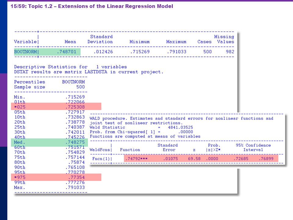
Bootstrap Estimation of the Asymptotic Variance of an Estimator
Known form of asymptotic variance: Compute from known results Unknown form, known generalities about properties: Use bootstrapping Root N consistency Sampling conditions amenable to central limit theorems Compute by resampling mechanism within the sample.

10
Bootstrapping Algorithm
1. Estimate parameters using full sample: b 2. Repeat R times: Draw n observations from the n, with replacement Estimate with b(r). 3. Estimate variance with V = (1/R)r [b(r) - b][b(r) - b]’ (Some use mean of replications instead of b. Advocated (without motivation) by original designers of the method.)
. 3. Estimate variance with V = (1/R)r [b(r) - b][b(r) - b]’ (Some use mean of replications instead of b. Advocated (without motivation) by original designers of the method.)")
11
Application: Correlation between Age and Education

12
Bootstrapped Regression

13
Bootstrap Replications

14
Bootstrapped Confidence Intervals Estimate Norm()=(12 + 22 + 32 + 42)1/2
=(12 + 22 + 32 + 42)1/2")
16
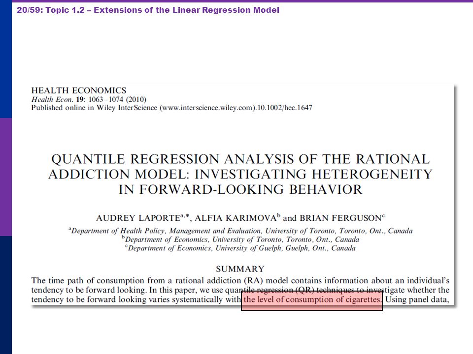
Quantile Regression Q(y|x,) = x, = quantile
Estimated by linear programming Q(y|x,.50) = x, .50 median regression Median regression estimated by LAD (estimates same parameters as mean regression if symmetric conditional distribution) Why use quantile (median) regression? Semiparametric Robust to some extensions (heteroscedasticity?) Complete characterization of conditional distribution
 = x, .50 median regression. Median regression estimated by LAD (estimates same parameters as mean regression if symmetric conditional distribution) Why use quantile (median) regression Semiparametric. Robust to some extensions (heteroscedasticity ) Complete characterization of conditional distribution.")
17
Estimated Variance for Quantile Regression

18
Quantile Regressions = .25 = .50 = .75

19
OLS vs. Least Absolute Deviations

21
Coefficient on MALE dummy variable in quantile regressions

22
A Production Function Model with Inefficiency The Stochastic Frontier Model

23
Inefficiency in Production

24
Cost Inefficiency y* = f(x) C* = g(y*,w) (Samuelson – Shephard duality results) Cost inefficiency: If y < f(x), then C must be greater than g(y,w). Implies the idea of a cost frontier. lnC = lng(y,w) + u, u > 0.
 C* = g(y*,w) (Samuelson – Shephard duality results) Cost inefficiency: If y < f(x), then C must be greater than g(y,w). Implies the idea of a cost frontier. lnC = lng(y,w) + u, u > 0.")
25
Corrected Ordinary Least Squares

26
COLS Cost Frontier

27
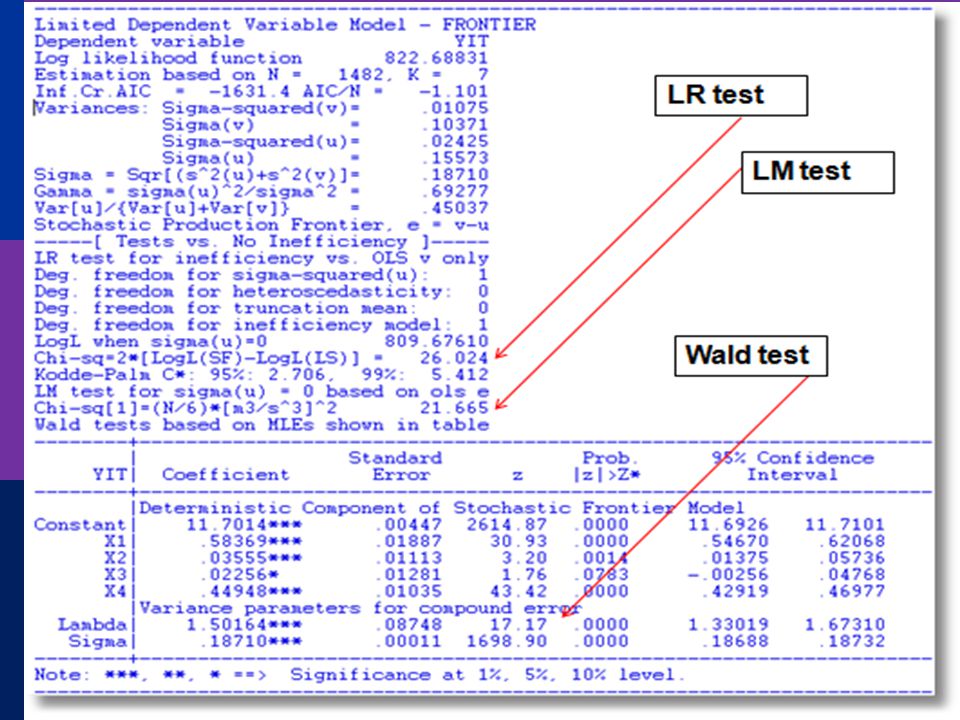
Stochastic Frontier Models
Motivation: Factors not under control of the firm Measurement error Differential rates of adoption of technology Frontier is randomly placed by the whole collection of stochastic elements which might enter the model outside the control of the firm. Aigner, Lovell, Schmidt (1977), Meeusen, van den Broeck (1977), Battese, Corra (1977)
, Meeusen, van den Broeck (1977), Battese, Corra (1977)")
28
The Stochastic Frontier Model
ui > 0, but vi may take any value. A symmetric distribution, such as the normal distribution, is usually assumed for vi. Thus, the stochastic frontier is +’xi+vi and, as before, ui represents the inefficiency.

29
Least Squares Estimation
Average inefficiency is embodied in the third moment of the disturbance εi = vi - ui. So long as E[vi - ui] is constant, the OLS estimates of the slope parameters of the frontier function are unbiased and consistent. (The constant term estimates α-E[ui]. The average inefficiency present in the distribution is reflected in the asymmetry of the distribution, which can be estimated using the OLS residuals:

30
Application to Spanish Dairy Farms
N = 247 farms, T = 6 years ( ) Input Units Mean Std. Dev. Minimum Maximum Milk Milk production (liters) 131,108 92,539 14,110 727,281 Cows # of milking cows 2.12 11.27 4.5 82.3 Labor # man-equivalent units 1.67 0.55 1.0 4.0 Land Hectares of land devoted to pasture and crops. 12.99 6.17 2.0 45.1 Feed Total amount of feedstuffs fed to dairy cows (tons) 57,941 47,981 3,924.14 376,732
 Input. Units. Mean. Std. Dev. Minimum. Maximum. Milk. Milk production (liters) 131, , , ,281. Cows. # of milking cows Labor. # man-equivalent units Land. Hectares of land devoted to pasture and crops Feed. Total amount of feedstuffs fed to dairy cows (tons) 57, ,981. 3, ,732.")
31
Example: Dairy Farms

32
The Normal-Half Normal Model

33
Skew Normal Variable

34
Estimation: Least Squares/MoM
OLS estimator of β is consistent E[ui] = (2/π)1/2σu, so OLS constant estimates α+ (2/π)1/2σu Second and third moments of OLS residuals estimate Method of Moments: Use [a,b,m2,m3] to estimate [,,u, v]
1/2σu, so OLS constant estimates α+ (2/π)1/2σu. Second and third moments of OLS residuals estimate. Method of Moments: Use [a,b,m2,m3] to estimate [,,u, v]")
35
Standard Form: The Skew Normal Distribution

36
Log Likelihood Function
Waldman (1982) result on skewness of OLS residuals: If the OLS residuals are positively skewed, rather than negative, then OLS maximizes the log likelihood, and there is no evidence of inefficiency in the data.
 result on skewness of OLS residuals: If the OLS residuals are positively skewed, rather than negative, then OLS maximizes the log likelihood, and there is no evidence of inefficiency in the data.")
37
Airlines Data – 256 Observations

38
Least Squares Regression

40
Alternative Models: Half Normal and Exponential

41
Normal-Exponential Likelihood
Other Models Many other parametric models Semiparametric and nonparametric – the recent outer reaches of the theoretical literature Other variations including heterogeneity in the frontier function and in the distribution of inefficiency

42
A Test for Inefficiency?
Base test on u = 0 <=> = 0 Standard test procedures Likelihood ratio Wald Lagrange Multiplier Nonstandard testing situation: Variance = 0 on the boundary of the parameter space Standard chi squared distribution does not apply.

44
Estimating ui No direct estimate of ui
Data permit estimation of yi – β’xi. Can this be used? εi = yi – β’xi = vi – ui Indirect estimate of ui, using E[ui|vi – ui] This is E[ui|yi, xi] vi – ui is estimable with ei = yi – b’xi.

45
Fundamental Tool - JLMS
We can insert our maximum likelihood estimates of all parameters. Note: This estimates E[u|vi – ui], not ui.

46
Application: Electricity Generation

47
Estimated Translog Production Frontiers

48
Inefficiency Estimates

49
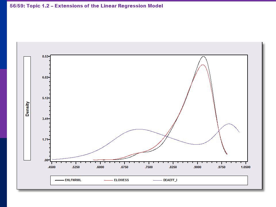
Estimated Inefficiency Distribution

50
Estimated Efficiency

51
A Semiparametric Approach
Y = g(x,z) + v - u [Normal-Half Normal] (1) Locally linear nonparametric regression estimates g(x,z) (2) Use residuals from nonparametric regression to estimate variance parameters using MLE (3) Use estimated variance parameters and residuals to estimate technical efficiency.
 + v - u [Normal-Half Normal] (1) Locally linear nonparametric regression estimates g(x,z) (2) Use residuals from nonparametric regression to estimate variance parameters using MLE (3) Use estimated variance parameters and residuals to estimate technical efficiency.")
52
Airlines Application

53
Efficiency Distributions

54
Nonparametric Methods - DEA

55
DEA is done using linear programming

57
Methodological Problems with DEA
Measurement error Outliers Specification errors The overall problem with the deterministic frontier approach

58
DEA and SFA: Same Answer?
Christensen and Greene data N=123 minus 6 tiny firms X = capital, labor, fuel Y = millions of KWH Cobb-Douglas Production Function vs. DEA

60
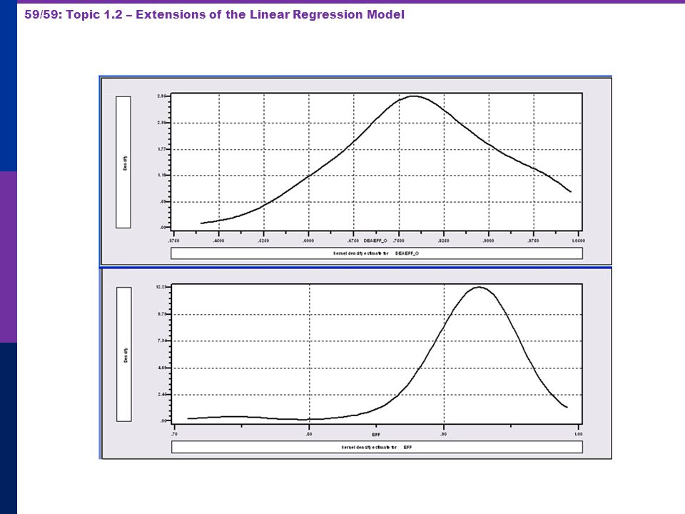
Comparing the Two Methods.

Similar presentations


![[Part 3] 1/49 Stochastic FrontierModels Stochastic Frontier Model Stochastic Frontier Models William Greene Stern School of Business New York University.](/15/4666432/big_thumb.jpg "[Part 3] 1/49 Stochastic FrontierModels Stochastic Frontier Model Stochastic Frontier Models William Greene Stern School of Business New York University.>")


>")


