1. Lecture 11: Transformations CS4670/5760: Computer Vision Kavita Bala

2. Announcements HW 1 FAQ pinned on Piazza PA 1 Artifacts – Soon voting will be set up. Please vote PA 2 out this weekend – Will present in class on Monday Next Friday: in class review Prelim: Mar 5, Thu, 7:30pm – Call Auditorium, Kennedy Hall

3. Reading Szeliski: Chapter 6.1, 3.6

4. What is the geometric relationship between these two images? ? Answer: Similarity transformation (translation, rotation, uniform scale)

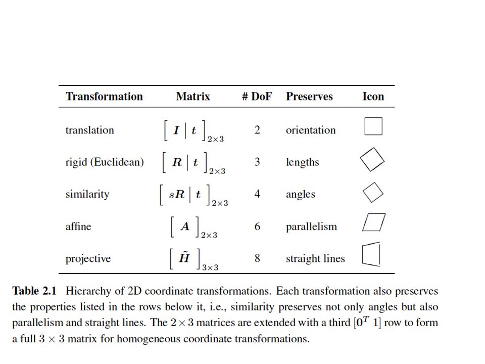
5. All 2D Linear Transformations Linear transformations are combinations of … – Scale, – Rotation, – Shear, and – Mirror Properties of linear transformations: – Origin maps to origin – Lines map to lines – Parallel lines remain parallel – Ratios are preserved – Closed under composition

6. Homogeneous coordinates Trick: add one more coordinate: homogeneous image coordinates Converting from homogeneous coordinates x y w (x, y, w) w = 1 (x/w, y/w, 1) homogeneous plane

7. Translation Solution: homogeneous coordinates to the rescue

8. Affine transformations any transformation with last row [ 0 0 1 ] we call an affine transformation

9. Basic affine transformations Translate 2D in-plane rotationShear Scale

10. Affine Transformations Affine transformations are combinations of … – Linear transformations, and – Translations Properties of affine transformations: – Origin does not necessarily map to origin – Lines map to lines – Parallel lines remain parallel – Ratios are preserved – Closed under composition

11. Euclidean: translation, rotation, reflection Similarity: translation, rotation, uniform scale, reflection Affine: linear transformations + translation

13. 2D image transformations These transformations are a nested set of groups Closed under composition and inverse is a member

14. Homographies

15. Reading Szeliski: Chapter 3.6

16. Is this an affine transformation?

17. Where do we go from here? affine transformation what happens when we mess with this row?

18. Projective Transformations aka Homographies aka Planar Perspective Maps Called a homography (or planar perspective map)

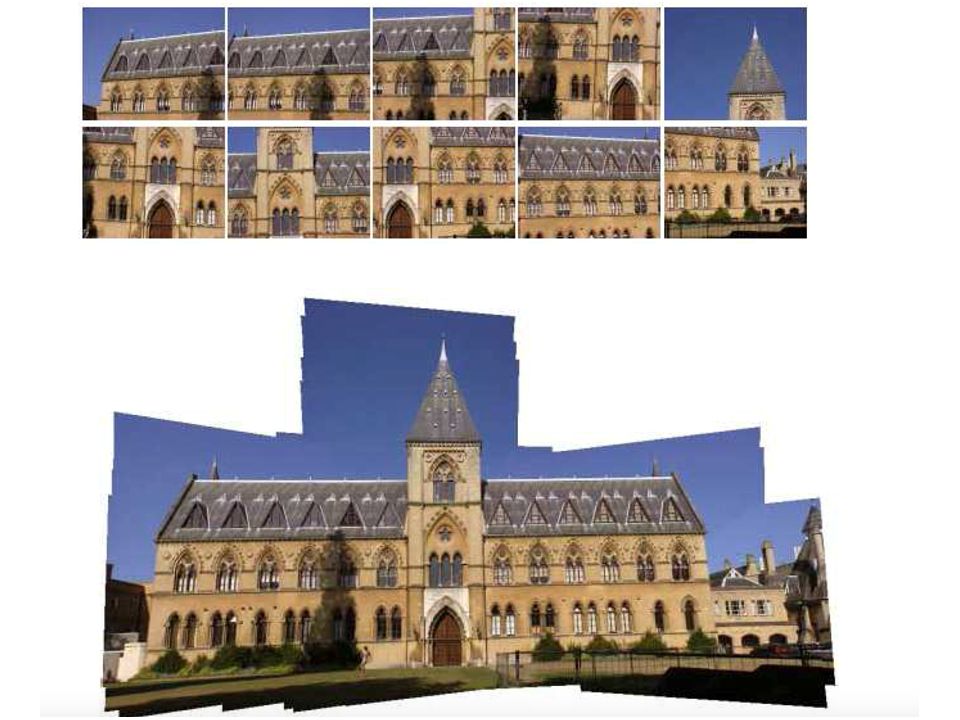
19. Why do we care? What is the relation between a plane in the world and a perspective image of it? Can we reconstruct another view from one image? Relation between pairs of images – Need to make a mosaic

21. Homographies

22. Recap of 4620

23. Plane projection in drawing [CS 417 Spring 2002] 23

24. Perspective projection similar triangles: (y’, f) (x’, y’, w’) = (fx, fy, z) x’ = fx/z, y’ = fy/z

25. Homographies

26. What happens when the denominator is 0?

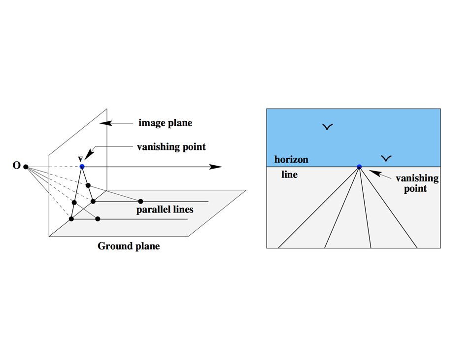
27. Points at infinity

28. Implications of w All scalar multiples of a 4-vector are equivalent When w is not zero, can divide by w – therefore these points represent “normal” affine points When w is zero, it’s a point at infinity, a.k.a. a direction – this is the point where parallel lines intersect – can also think of it as the vanishing point 28

29. 29 Masaccio, Trinity, Florence

31. Consider a line through point (a, b) with slope m x’ = a + m t (line through a along direction m) if t = 1/w; x’ = (a w + m)/w In homogeneous coordinates (aw+m, w) At w = 0, point at infinity (m,0) represents line with slope m 31

32. Image warping with homographies image plane in frontimage plane below black area where no pixel maps to

33. Homographies

34. Homographies … – Affine transformations, and – Projective warps Properties of projective transformations: – Origin does not necessarily map to origin – Lines map to lines – Parallel lines do not necessarily remain parallel – Ratios are not preserved – Closed under composition

35. 2D image transformations These transformations are a nested set of groups Closed under composition and inverse is a member

37. Image Warping Given a coordinate xform (x’,y’) = T(x,y) and a source image f(x,y), how do we compute an xformed image g(x’,y’) = f(T(x,y))? f(x,y)g(x’,y’) xx’ T(x,y) y y’

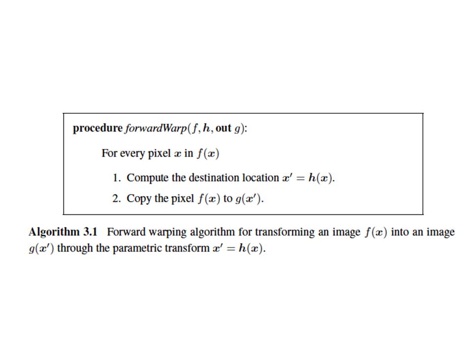
38. Forward Warping Send each pixel f(x) to its corresponding location (x’,y’) = T(x,y) in g(x’,y’) f(x,y)g(x’,y’) xx’ T(x,y) y y’

40. Forward Warping Send each pixel f(x,y) to its corresponding location x’ = h(x,y) in g(x’,y’) f(x,y)g(x’,y’) xx’ T(x,y) What if pixel lands “between” pixels? Answer: add “contribution” to several pixels, normalize later (splatting) Problem? Can still result in holes y y’

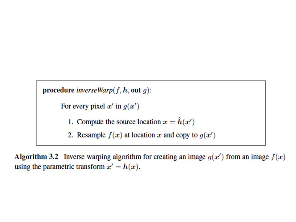
41. Inverse Warping Get each pixel g(x’,y’) from its corresponding location (x,y) = T -1 (x,y) in f(x,y) f(x,y)g(x’,y’) xx’ T -1 (x,y) Requires taking the inverse of the transform What if pixel comes from “between” pixels? y y’

42. Inverse Warping Get each pixel g(x’) from its corresponding location x’ = h(x) in f(x) What if pixel comes from “between” two pixels? Answer: resample color value from interpolated (prefiltered) source image f(x,y)g(x’,y’) xx’ y y’ T -1 (x,y)

44. Interpolation Possible interpolation filters: – nearest neighbor – bilinear – bicubic (interpolating) – sinc Needed to prevent “jaggies” and “texture crawl” (with prefiltering)