1. Financial and Managerial Accounting
Preview of Chapter 19
Financial and Managerial Accounting
Weygandt Kimmel Kieso

2. Cost Behavior Analysis
Cost Behavior Analysis … how costs react to changes in the level of business activity.
Some costs change; others remain the same.
Activity levels (Activity Index) may be: Sales Dollars, % Occupancy, # Covers, # Miles, # Classes
Allows costs to be classified as: variable, fixed, or mixed (part fixed part variable).

3. Variable costs vary in total, stay the same per unit.
Cost Behavior Analysis
Variable Costs
Costs that vary in total directly and proportionately with changes in the activity level.
Activity up 10%, then total variable costs go up 10% Activity down 25%, then total variable cost go down 25%.
Variable costs remain the same per unit regardless.
Variable costs vary in total, stay the same per unit.

4. Cost Behavior Analysis
Illustration: iMac uses a $10 camera. Activity index is the # of
computers produced. For each iMac iMac made (per unit), the total cost of the camera increases by $10.
Total Cost of the cameras will be: * $20,000 if 2,000 iMacs are made, * $100,000 when it makes 10,000.

5. Cost Behavior Analysis
Illustration: iMac uses a $10 camera. Activity index is the # of
computers produced. For each iMac iMac made (per unit), the total cost of the camera increases by $10.
“Per Unit” Cost of $10 for each camera remains constant (the same) whether 2,000 or 10,000 iMacs are produced.

6. Cost Behavior Analysis
Variable Costs “Behavior”

7. Cost Behavior Analysis
Fixed Costs
Costs that remain the same in total regardless of changes in the activity level.
Per unit cost varies inversely with activity: As volume goes up, unit cost goes down, As volume goes down, unit costs go up
Examples:
Property taxes … Insurance … Rent
Depreciation on buildings and equipment

8. Cost Behavior Analysis
Illustration: Apple leases (rents) a factory building at a cost of $10,000 per month.
Total fixed costs for the factory rent will remain constant (the same) at every level of activity.
Ex: manufacture 1 or 10,000 iMacs, the factory rent costs is $10,000.

9. Cost Behavior Analysis
Illustration: Apple leases (rents) a factory building at a cost of $10,000 per month.
Cost per unit decreases as activity increases.
When 2,000 iMacs are made, the unit cost per iMac = $5 ($10,000 ÷ 2,000).
When 10,000 iMacs are made, the unit cost = $1 ($10,000 ÷ 10,000).

10. Cost Behavior Analysis
Fixed Costs “Behavior”

11. Cost Behavior Analysis
Relevant Range
Throughout the range of possible levels of activity, a straight-line relationship usually does not exist for either variable costs or fixed costs.
Relationship between variable costs and changes in activity level is often curvilinear.
For fixed costs, the relationship is also nonlinear – some fixed costs will not change over the entire range of activities, while other fixed costs may change.

12. Cost Behavior Analysis
Relevant Range

13. Cost Behavior Analysis
Relevant Range … Range of activity (“how busy”) a company expects to operate during a year. (normal or usual)

14. Cost Behavior Analysis
Mixed Costs
Costs with both variable and fixed cost elements.
Change in total … but not proportionately with changes in activity.
Ex: car rental: $20 per day (fixed) PLUS .10 per mile (variable)

15. Assume your weekly pay is based on % of everything that you sell.
Day
# Sold
$ Earned
Mon 10 50
Tues
Wed 13 65
Thurs
Fri 17 85
Sat 24
120
Sun 21
105

16. Assume your weekly pay is based on salary + commission.
Day
# Sold
$ Earned
Mon 10 70
Tues 20
Wed 13 85
Thurs
Fri 17
105
Sat 24
140
Sun 21
125

17. Cost Behavior Analysis
High-Low Method
Mixed costs must be classified into their fixed and variable elements.
High-Low uses the total costs incurred at both the high and the low levels of activity to classify mixed costs.
The difference in costs between the high and low levels represents variable costs, since only variable costs change as activity levels change.

18. Cost Behavior Analysis
High-Low Method
STEP 1: Determine variable cost per unit using formula:
Day
# Sold
$ Earned
Mon 10 70
Tues 20
Wed 13 85
Thurs
Fri 17
105
Sat 24
140
Sun 21
125
(High$ – Low$)
HighSold - LowSold
140
-20
120 20 -0 $
120 20
= $ per unit
units

19. Cost Behavior Analysis
High-Low Method
Illustration: Metro Bus Co. has these maintenance costs and mileage data for its fleet of buses over a 6-month period.

20. Cost Behavior Analysis
High-Low Method
STEP 2: fixed cost - total variable cost at either the high or low activity level.

21. Cost Behavior Analysis
High-Low Method
Maintenance costs = $8,000 per month plus $1.10 per mile. (Represented by formula):
Maintenance costs = Fixed costs + ($1.10 x Miles driven)
Ex: At 45,000 miles, estimated maintenance costs would be:
Fixed
$ 8,000
Variable
($1.10 x 45,000) 49,500
$57,500

22. Cost Behavior Analysis
Mixed Costs “Behavior”
Note that costs START at $8,000

23. Byrnes Company accumulates the following data concerning a mixed cost, using units produced as the activity level.
Compute the variable and fixed cost elements using the high-low method.
Estimate the total cost if the company produces 6,000 units.

24. Compute the variable and fixed cost elements using the high-low method.
Variable cost: ($14,740 - $11,100) / (9, ,000) = $1.30 per unit
Fixed cost: $14,740 - $12,740 ($1.30 x 9,800 units) = $2,000
or $11,100 - $9,100 ($1.30 x 7,000) = $2,000

25. Estimate the total cost if the company produces 6,000 units.
Total cost (6,000 units): $2,000 + $7,800 ($1.30 x 6,000) = $9,800

27. Cost-Volume-Profit Analysis
Cost-volume-profit (CVP) analysis is the study of the effects of changes of costs and volume on a company’s profits.
Important in profit planning
Critical factor in management decisions as
Setting selling prices,
Determining product mix, and
Maximizing use of production facilities.

28. Cost-Volume-Profit Analysis
Basic Components
Illustration 19-9

29. Cost-Volume-Profit Analysis
Basic Components - Assumptions
Behavior of both costs and revenues is linear throughout the relevant range of the activity index.
All costs can be classified as either variable or fixed with reasonable accuracy.
Changes in activity are the only factors that affect costs.
All units produced are sold.
When more than one type of product is sold, the sales mix will remain constant.

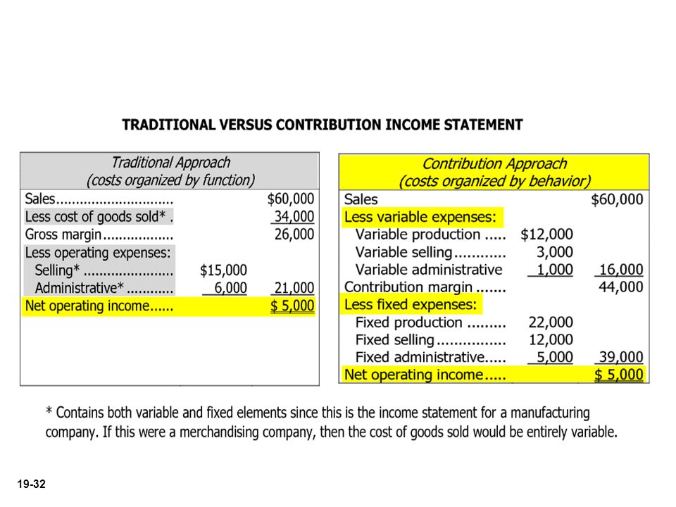
30. Traditional Income Statement GAAP required for external reporting
(Revenue – Expenses = Net Income)
GAAP required for external reporting

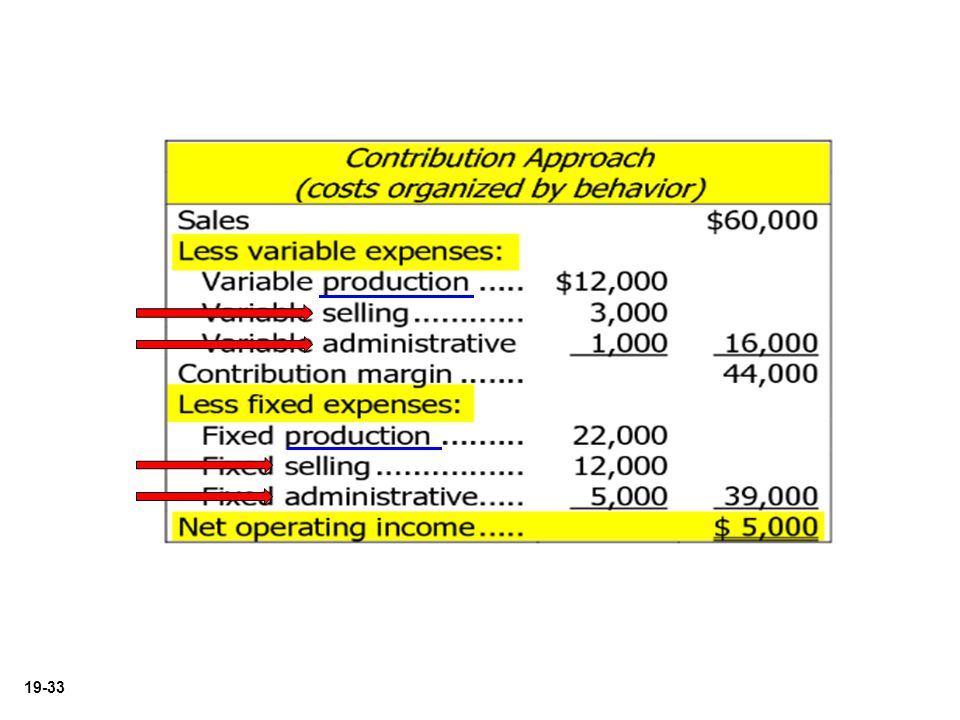
31. Cost-Volume-Profit Analysis
CVP Income Statement
A statement for internal use.
Classifies costs and expenses as fixed or variable.
Reports contribution margin in the statement.
Contribution margin – amount of revenue remaining after deducting variable costs.
Same net income as a traditional income statement.

34. Cost-Volume-Profit Analysis
CVP Income Statement
Illustration: Vargo Video produces a high-definition digital camcorder. Relevant data for June 2014 are as follows.

35. Cost-Volume-Profit Analysis
CVP Income Statement
Illustration: The CVP income statement would be:

36. Cost-Volume-Profit Analysis
Contribution Margin per Unit
Contribution Margin must cover ALL fixed costs THEN profit (which is the “contribution” to net income).

37. Cost-Volume-Profit Analysis
Contribution Margin per Unit
Vargo’s CVP income statement assuming a zero net income.

38. Cost-Volume-Profit Analysis
Contribution Margin per Unit
WHAT IF … sell one more unit, (1,001 vs 1,000 units sold).

39. Break-Even Point When Revenue exactly equals ALL costs
(Revenue – Variable – Fixed Expenses = Breakeven Point)
Where loss ends and profit begins.
The point at which a business, product or project becomes financially viable.
Expressed as “Dollars” or “Units”.

40. Cost-Volume-Profit Analysis
Break-Even Analysis
Process of finding the break-even point where total revenues equal total costs (both fixed and variable).
Can be computed or derived
from a mathematical equation,
by using contribution margin, or
from a cost-volume profit (CVP) graph.
Expressed either in sales units or in sales dollars.

41. Break-Even Analysis Mathematical Equation
Break-even occurs where total sales equal variable costs plus fixed costs; i.e., net income is zero
Computation of break-even point in units.
Illustration 19-20

42. Cost-Volume-Profit Analysis
Contribution Margin Ratio
Shows the percentage of each sales dollar available to apply toward fixed costs and profits.
Formula for contribution margin ratio is:

43. Cost-Volume-Profit Analysis
Contribution Margin Ratio
If current sales are $500,000 what is the effect of a $100,000 (200-unit) increase in sales.

44. Break-Even Analysis Contribution Margin Technique
When the BEP in units is desired, contribution margin per unit is used in the following formula:

45. Break-Even Analysis Contribution Margin Technique
When the BEP in dollars is desired, contribution margin ratio is used in the following formula:

46. Break-Even Analysis Graphic Presentation
Because this graph also shows costs, volume, and profits, it is referred to as a cost-volume-profit (CVP) graph.

47. Cost-Volume-Profit Analysis
Target Net Income
Sales necessary to achieve a specified income.
Can be determined from any approaches used to determine break-even sales/units:
from a mathematical equation,
by using contribution margin, or
from a cost-volume profit (CVP) graph.

48. Cost-Volume-Profit Analysis
Target Net Income
Sales necessary to achieve a specified level of income.
Mathematical Equation
Formula for required sales to meet target net income.

49. Target Net Income Mathematical Equation
Using the formula for the break-even point, simply include the desired net income as a factor.
Illustration 19-25

50. Target Net Income Contribution Margin Technique
To determine the required sales in units for Vargo Video:
Illustration 19-26

51. Target Net Income Contribution Margin Technique
To determine the required sales in dollars for Vargo Video:
Illustration 19-27

52. Cost-Volume-Profit Analysis
Margin of Safety
Difference between actual (or projected) sales and the sales at the break-even point.
Measures the “cushion” if expected sales fail to materialize.
May be expressed in dollars or as a ratio.
Assuming actual/expected sales are $750,000:

53. Cost-Volume-Profit Analysis
Margin of Safety Ratio
Divide the margin of safety in $$ by the actual or sales.
Assuming actual/expected sales are $750,000:
The higher the dollars or %, the greater the margin of safety.