1. Planning Subbarao Kambhampati 11/2/2009

2. Environment What action next? The $$$$$$ Question

3. Environment action perception Goals (Static vs. Dynamic) (Observable vs. Partially Observable) (perfect vs. Imperfect) (Deterministic vs. Stochastic) What action next? (Instantaneous vs. Durative) (Full vs. Partial satisfaction) The $$$$$$ Question

4. The representational roller-coaster in CSE 471 atomic propositional/ (factored) relational First-order State-space search CSPProp logicBayes Nets FOPC w.o. functions FOPCSit. Calc. STRIS Planning MDPsMin-max Decision trees Semester time  The plot shows the various topics we discussed this semester, and the representational level at which we discussed them. At the minimum we need to understand every task at the atomic representation level. Once we figure out how to do something at atomic level, we always strive to do it at higher (propositional, relational, first-order) levels for efficiency and compactness. During the course we may not discuss certain tasks at higher representation levels either because of lack of time, or because there simply doesn’t yet exist undergraduate level understanding of that topic at higher levels of representation..

5. Why go for higher level models? Ease of specification –Ease of acquisition Either by you interviewing expers Or your program learning –(did you ever wonder why there is no “atomic” level learning? We assume that examples must be describable in terms of features, at the very least..) Ease of inference –More interesting kinds of search »(e.g. Regression search corresponds to multiple parallel backward state searches) –More automated ways of deriving heuristics to guide the search

6. Applications—sublime and mundane Mission planning (for rovers, telescopes) Military planning/scheduling Web-service/Work-flow composition Paper-routing in copiers Gene regulatory network intervention

7. Deterministic Planning Given an initial state I, a goal state G and a set of actions A:{a1…an} Find a sequence of actions that when applied from the initial state will lead the agent to the goal state. Qn: Why is this not just a search problem (with actions being operators?) –Answer: We have “factored” representations of states and actions. And we can use this internal structure to our advantage in –Formulating the search (forward/backward/insideout) –deriving more powerful heuristics etc.

8. Blocks world State variables: Ontable(x) On(x,y) Clear(x) hand-empty holding(x) Stack(x,y) Prec: holding(x), clear(y) eff: on(x,y), ~cl(y), ~holding(x), hand-empty Unstack(x,y) Prec: on(x,y),hand-empty,cl(x) eff: holding(x),~clear(x),clear(y),~hand-empty Pickup(x) Prec: hand-empty,clear(x),ontable(x) eff: holding(x),~ontable(x),~hand-empty,~Clear(x) Putdown(x) Prec: holding(x) eff: Ontable(x), hand-empty,clear(x),~holding(x) Initial state: Complete specification of T/F values to state variables --By convention, variables with F values are omitted Goal state: A partial specification of the desired state variable/value combinations --desired values can be both positive and negative Init: Ontable(A),Ontable(B), Clear(A), Clear(B), hand-empty Goal: ~clear(B), hand-empty All the actions here have only positive preconditions; but this is not necessary STRIPS ASSUMPTION: If an action changes a state variable, this must be explicitly mentioned in its effects

9. State Variable Models World is made up of states which are defined in terms of state variables –Can be boolean (or multi-ary or continuous) States are complete assignments over state variables –So, k boolean state variables can represent how many states? Actions change the values of the state variables –Applicability conditions of actions are also specified in terms of partial assignments over state variables

10. Why is STRIPS representation compact? (than explicit transition systems) In explicit transition systems actions are represented as state-to-state transitions where in each action will be represented by an incidence matrix of size |S|x|S| In state-variable model, actions are represented only in terms of state variables whose values they care about, and whose value they affect. Consider a state space of 1024 states. It can be represented by log 2 1024=10 state variables. If an action needs variable v1 to be true and makes v7 to be false, it can be represented by just 2 bits (instead of a 1024x1024 matrix) –Of course, if the action has a complicated mapping from states to states, in the worst case the action rep will be just as large –The assumption being made here is that the actions will have effects on a small number of state variables. Sit. Calc STRIPS rep Transition rep First order Rel/ Prop Atomic Glass is half-full

11. What do we lose with STRIPS actions? Need to write all effects explicitly –Can’t depend on derived effects Leads to loss of modularity –Instead of saying “Clear” holds when nothing is “On” the block, we have to write Clear effects everywhere –If now the blocks become bigger and can hold two other blocks, you will have to rewrite all the action descriptions Then again, state-variable (STRIPS) model is a step- up from the even more low-level “State Transition model” Where actions are just mappings from States to States (and so must be seen as SXS matrices) Very loose Analogy: State-transition models  Assembly lang (factored) state-variable models  C (first-order) sit-calc models  Lisp Glass is half-empty

12. How to do search with STRIPS models? Idea 1: Convert them back to transition models Idea 2: Use them directly..

13. Progression: An action A can be applied to state S iff the preconditions are satisfied in the current state The resulting state S’ is computed as follows: --every variable that occurs in the actions effects gets the value that the action said it should have --every other variable gets the value it had in the state S where the action is applied Ontable(A) Ontable(B), Clear(A) Clear(B) hand-empty holding(A) ~Clear(A) ~Ontable(A) Ontable(B), Clear(B) ~handempty Pickup(A) Pickup(B) holding(B) ~Clear(B) ~Ontable(B) Ontable(A), Clear(A) ~handempty STRIPS ASSUMPTION: If an action changes a state variable, this must be explicitly mentioned in its effects

14. On the asymmetry of init/goal states Goal state is partial –It is a (seemingly) good thing if only m of the k state variables are mentioned in a goal specification, then upto 2 k-m complete state of the world can satisfy our goals!..I say “seeming” because sometimes a more complete goal state may provide hints to the agent as to what the plan should be –In the blocks world example, if we also state that On(A,B) as part of the goal (in addition to ~Clear(B)&hand-empty) then it would be quite easy to see what the plan should be.. Initial State is complete –If initial state is partial, then we have “partial observability” (i.e., the agent doesn’t know where it is!) If only m of the k state variables are known, then the agent is in one of 2 k-m states! In such cases, the agent needs a plan that will take it from any of these states to a goal state –Either this could be a single sequence of actions that works in all states (e.g. bomb in the toilet problem) –Or this could be “conditional plan” that does some limited sensing and based on that decides what action to do..More on all this during the third class Because of the asymmetry between init and goal states, progression is in the space of complete states, while regression is in the space of “partial” states (sets of states). Specifically, for k state variables, there are 2 k complete states and 3 k “partial” states –(a state variable may be present positively, present negatively or not present at all in the goal specification!)

15. Generic (progression) planner Goal test(S,G)—check if every state variable in S, that is mentioned in G, has the value that G gives it. Child generator(S,A) –For each action a in A do If every variable mentioned in Prec(a) has the same value in it and S –Then return Progress(S,a) as one of the children of S »Progress(S,A) is a state S’ where each state variable v has value v[Eff(a)]if it is mentioned in Eff(a) and has the value v[S] otherwise Search starts from the initial state

16. Regression: A state S can be regressed over an action A (or A is applied in the backward direction to S) Iff: --There is no variable v such that v is given different values by the effects of A and the state S --There is at least one variable v’ such that v’ is given the same value by the effects of A as well as state S The resulting state S’ is computed as follows: -- every variable that occurs in S, and does not occur in the effects of A will be copied over to S’ with its value as in S -- every variable that occurs in the precondition list of A will be copied over to S’ with the value it has in in the precondition list ~clear(B) hand-empty Putdown(A) Stack(A,B) ~clear(B) holding(A) clear(B) Putdown(B)?? Termination test: Stop when the state s’ is entailed by the initial state s I *Same entailment dir as before..

17. Interpreting progression and regression in the transition graph In the transition graph (corresponding to the atomic model) –progression search corresponds to finding a single path –Regression search corresponds to simultaneously starting from multiple states (all of which satisfy the goal conditions), and effectively searching in parallel until one of the paths reaches the initial state Alternately, you can see regression as searching in the space of sets of states, with the termination condition being that any of the states is an initial state.

18. Heuristics for Planning 11/4 Qn: So which is better? Progression or Regression?

19. And now for an infomercial.. CSE494/598 in Spring 2010 Information Retrieval, Mining and Integration on the Internet T/Th 10:30—11:45. In this very room!..an easy A+

21. Progression vs. Regression The never ending war.. Part 1 Progression has higher branching factor Progression searches in the space of complete (and consistent) states Regression has lower branching factor Regression searches in the space of partial states –There are 3 n partial states (as against 2 n complete states) You can also do bidirectional search stop when a (leaf) state in the progression tree entails a (leaf) state (formula) in the regression tree

22. Regression vs. Reversibility Notice that regression doesn’t require that the actions are reversible in the real world –We only think of actions in the reverse direction during simulation –…just as we think of them in terms of their individual effects during partial order planning Normal blocks world is reversible (if you don’t like the effects of stack(A,B), you can do unstack(A,B)). However, if the blocks world has a “bomb” the table action, then normally, there won’t be a way to reverse the effects of that action. –But even with that action we can do regression –For example we can reason that the best way to make table go- away is to add “Bomb” action into the plan as the last action..although it might also make you go away

23. Planning vs. Search: What is the difference? Search assumes that there is a child-generator and goal-test functions which know how to make sense of the states and generate new states Planning makes the additional assumption that the states can be represented in terms of state variables and their values –Initial and goal states are specified in terms of assignments over state variables Which means goal-test doesn’t have to be a blackbox procedure –That the actions modify these state variable values The preconditions and effects of the actions are in terms of partial assignments over state variables –Given these assumptions certain generic goal-test and child-generator functions can be written Specifically, we discussed one Child-generator called “Progression”, another called “Regression” and a third called “Partial-order” Notice that the additional assumptions made by planning do not change the search algorithms (A*, IDDFS etc)—they only change the child-generator and goal-test functions –In particular, search still happens in terms of search nodes that have parent pointers etc. The “state” part of the search node will correspond to –“Complete state variable assignments” in the case of progression –“Partial state variable assignments” in the case of regression –“A collection of steps, orderings, causal commitments and open-conditions in the case of partial order planning

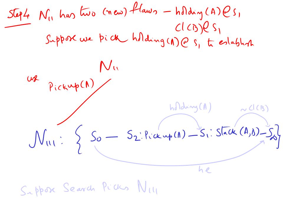
24. Plan Space Planning: Terminology Step: a step in the partial plan—which is bound to a specific action Orderings: s1<s2 s1 must precede s2 Open Conditions: preconditions of the steps (including goal step) Causal Link (s1—p—s2): a commitment that the condition p, needed at s2 will be made true by s1 –Requires s1 to “cause” p Either have an effect p Or have a conditional effect p which is FORCED to happen –By adding a secondary precondition to S1 Unsafe Link: (s1—p—s2; s3) if s3 can come between s1 and s2 and undo p (has an effect that deletes p). Empty Plan: { S:{I,G}; O:{I<G}, OC:{g1@G;g2@G..}, CL:{}; US:{}}

25. Algorithm 1. Let P be an initial plan 2. Flaw Selection: Choose a flaw f ( either open condition or unsafe link ) 3. Flaw resolution: If f is an open condition, choose an action S that achieves f If f is an unsafe link, choose promotion or demotion Update P Return NULL if no resolution exist 4. If there is no flaw left, return P else go to 2. S0S0 S1S1 S2S2 S3S3 S in f p ~p g1g1 g2g2 g2g2 oc 1 oc 2 q1q1 Choice points Flaw selection (open condition? unsafe link?) Flaw resolution (how to select (rank) partial plan?) Action selection (backtrack point) Unsafe link selection (backtrack point) S0S0 S inf g1g2g1g2 1. Initial plan: 2. Plan refinement (flaw selection and resolution): POP background

27. S_infty < S2

28. If it helps take away some of the pain, you may note that the remote agent used a form of partial order planner!

29. Relevance, Rechabililty & Heuristics Progression takes “applicability” of actions into account –Specifically, it guarantees that every state in its search queue is reachable..but has no idea whether the states are relevant (constitute progress towards top-level goals) SO, heuristics for progression need to help it estimate the “relevance” of the states in the search queue Regression takes “relevance” of actions into account –Specifically, it makes sure that every state in its search queue is relevant.. But has not idea whether the states (more accurately, state sets) in its search queue are reachable SO, heuristics for regression need to help it estimate the “reachability” of the states in the search queue Reachability: Given a problem [I,G], a (partial) state S is called reachable if there is a sequence [a 1,a 2,…,a k ] of actions which when executed from state I will lead to a state where S holds Relevance: Given a problem [I,G], a state S is called relevant if there is a sequence [a1,a2,…,ak] of actions which when executed from S will lead to a state satisfying (Relevance is Reachability from goal state) Since relevance is nothing but reachability from goal state, reachability analysis can form the basis for good heuristics

30. Subgoal interactions Suppose we have a set of subgoals G 1,….G n Suppose the length of the shortest plan for achieving the subgoals in isolation is l 1,….l n We want to know what is the length of the shortest plan for achieving the n subgoals together, l 1…n If subgoals are independent: l 1..n = l 1 +l 2 +…+l n If subgoals have +ve interactions alone: l 1..n < l 1 +l 2 +…+l n If subgoals have -ve interactions alone: l 1..n > l 1 +l 2 +…+l n If you made “independence” assumption, and added up the individual costs of subgoals, then your resultant heuristic will be  perfect if the goals are actually independent  inadmissible (over-estimating) if the goals have +ve interactions  un-informed (hugely under-estimating) if the goals have –ve interactions

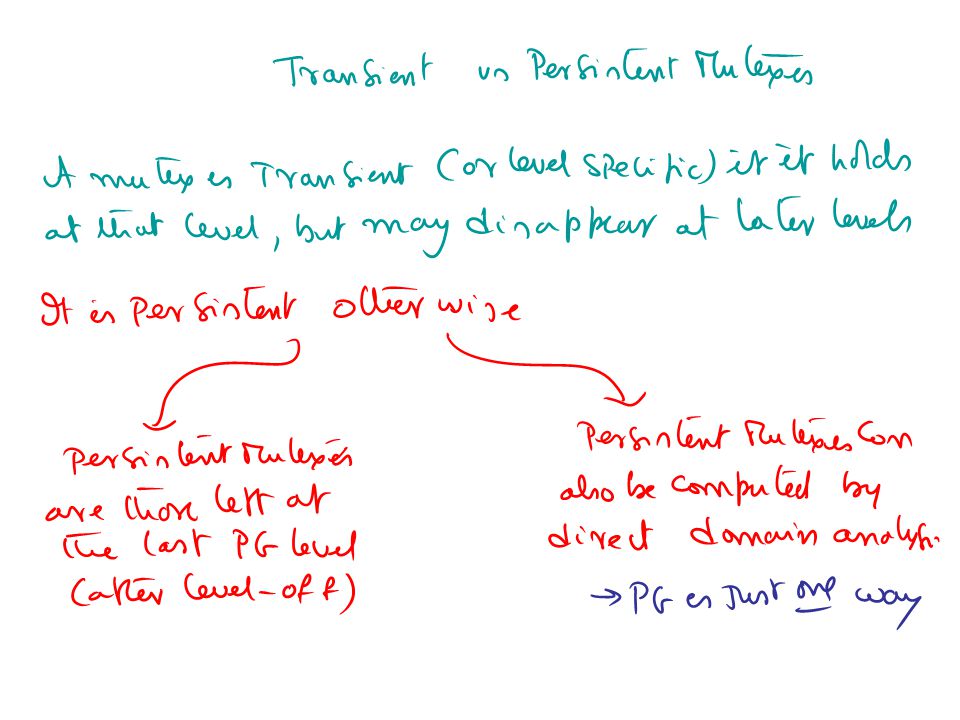
31. Planning Graph and Projection Envelope of Progression Tree (Relaxed Progression) –Proposition lists: Union of states at k th level –Mutex: Subsets of literals that cannot be part of any legal state Lowerbound reachability information [Blum&Furst, 1995] [ECP, 1997][AI Mag, 2007] p pq pr ps pqr pq pqs psq ps pst A1 A2 A3 A2 A1 A3 A1 A3 A4 p pqrspqrs pqrstpqrst A1 A2 A3 A1 A2 A3 A4 Planning Graphs can be used as the basis for heuristics!

32. Planning Graph Basics –Envelope of Progression Tree (Relaxed Progression) Linear vs. Exponential Growth –Reachable states correspond to subsets of proposition lists –BUT not all subsets are states Can be used for estimating non- reachability –If a state S is not a subset of k th level prop list, then it is definitely not reachable in k steps p pq pr ps pqr pq pqs p psq ps pst pqrspqrs pqrstpqrst A1 A2 A3 A2 A1 A3 A1 A3 A4 A1 A2 A3 A1 A2 A3 A4 [ECP, 1997]

34. Reachability through progression p pq pr ps pqr pq pqs psq ps pst A1 A2 A3 A2 A1 A3 A1 A3 A4 [ECP, 1997]

35. Planning Graph Basics –Envelope of Progression Tree (Relaxed Progression) Linear vs. Exponential Growth –Reachable states correspond to subsets of proposition lists –BUT not all subsets are states Can be used for estimating non- reachability –If a state S is not a subset of k th level prop list, then it is definitely not reachable in k steps p pq pr ps pqr pq pqs p psq ps pst pqrspqrs pqrstpqrst A1 A2 A3 A2 A1 A3 A1 A3 A4 A1 A2 A3 A1 A2 A3 A4 [ECP, 1997]

36. Scalability of Planning  Before, planning algorithms could synthesize about 6 – 10 action plans in minutes  Significant scale-up in the last 6-7 years  Now, we can synthesize 100 action plans in seconds. Realistic encodings of Munich airport! The primary revolution in planning in the recent years has been domain-independent heuristics to scale up plan synthesis Problem is Search Control!!! …and now for a ring-side retrospective

37. h set-difference hChC hPhP h*h* h0h0 Cost of computing the heuristic Cost of searching with the heuristic Total cost incurred in search Not always clear where the total minimum occurs Old wisdom was that the global min was closer to cheaper heuristics Current insights are that it may well be far from the cheaper heuristics for many problems E.g. Pattern databases for 8-puzzle Plan graph heuristics for planning Scalability came from sophisticated reachability heuristics based on planning graphs....and not from any hand-coded domain-specific control knoweldge “Optimistic projection of achievability”

38. Don’t look at curved lines for now… Have(cake) ~eaten(cake) ~Have(cake) eaten(cake) Eat No-op Have(cake) eaten(cake) bake ~Have(cake) eaten(cake) Have(cake) ~eaten(cake) Eat No-op Have(cake) ~eaten(cake) Graph has leveled off, when the prop list has not changed from the previous iteration The note that the graph has leveled off now since the last two Prop lists are the same (we could actually have stopped at the Previous level since we already have all possible literals by step 2)

39. Blocks world State variables: Ontable(x) On(x,y) Clear(x) hand-empty holding(x) Stack(x,y) Prec: holding(x), clear(y) eff: on(x,y), ~cl(y), ~holding(x), hand-empty Unstack(x,y) Prec: on(x,y),hand-empty,cl(x) eff: holding(x),~clear(x),clear(y),~hand-empty Pickup(x) Prec: hand-empty,clear(x),ontable(x) eff: holding(x),~ontable(x),~hand-empty,~Clear(x) Putdown(x) Prec: holding(x) eff: Ontable(x), hand-empty,clear(x),~holding(x) Initial state: Complete specification of T/F values to state variables --By convention, variables with F values are omitted Goal state: A partial specification of the desired state variable/value combinations --desired values can be both positive and negative Init: Ontable(A),Ontable(B), Clear(A), Clear(B), hand-empty Goal: ~clear(B), hand-empty All the actions here have only positive preconditions; but this is not necessary

40. onT-A onT-B cl-A cl-B he Pick-A Pick-B onT-A onT-B cl-A cl-B he h-A h-B ~cl-A ~cl-B ~he

41. onT-A onT-B cl-A cl-B he Pick-A Pick-B onT-A onT-B cl-A cl-B he h-A h-B ~cl-A ~cl-B ~he St-A-B St-B-A Ptdn-A Ptdn-B Pick-A onT-A onT-B cl-A cl-B he h-A h-B ~cl-A ~cl-B ~he on-A-B on-B-A Pick-B

42. Estimating the cost of achieving individual literals (subgoals) Idea: Unfold a data structure called “planning graph” as follows: 1. Start with the initial state. This is called the zeroth level proposition list 2. In the next level, called first level action list, put all the actions whose preconditions are true in the initial state -- Have links between actions and their preconditions 3. In the next level, called first level propostion list, put: Note: A literal appears at most once in a proposition list. 3.1. All the effects of all the actions in the previous level. Links the effects to the respective actions. (If multiple actions give a particular effect, have multiple links to that effect from all those actions) 3.2. All the conditions in the previous proposition list (in this case zeroth proposition list). Put persistence links between the corresponding literals in the previous proposition list and the current proposition list. *4. Repeat steps 2 and 3 until there is no difference between two consecutive proposition lists. At that point the graph is said to have “leveled off” The next 2 slides show this expansion upto two levels

44. Using the planning graph to estimate the cost of single literals: 1. We can say that the cost of a single literal is the index of the first proposition level in which it appears. --If the literal does not appear in any of the levels in the currently expanded planning graph, then the cost of that literal is: -- l+1 if the graph has been expanded to l levels, but has not yet leveled off -- Infinity, if the graph has been expanded (basically, the literal cannot be achieved from the current initial state) Examples: h({~he}) = 1 h ({On(A,B)}) = 2 h({he})= 0 How about sets of literals?  see next slide

45. Estimating reachability of sets We can estimate cost of a set of literals in three ways: Make independence assumption h sum (p,q,r)= h(p)+h(q)+h(r) if we define the cost of a set of literals in terms of the level where they appear together h-lev({p,q,r})= The index of the first level of the PG where p,q,r appear together so, h({~he,h-A}) = 1 Compute the length of a “relaxed plan” to supporting all the literals in the set S, and use it as the heuristic (**) h relax

46. Neither h lev nor h sum work well always p1p1 p2p2 p3p3 p 99 p 100 B1 q B2 B3 B99 B100 q P1P1 A0A0 P0P0 p1p1 p2p2 p3p3 p 99 p 100 q B* q P1P1 A0A0 P0P0 True cost of {p 1 …p 100 } is 100 (needs 100 actions to reach) H lev says the cost is 1 H sum says the cost is 100 H sum better than H lev True cost of {p 1 …p 100 } is 1 (needs just one action reach) H lev says the cost is 1 H sum says the cost is 100 H lev better than H sum H relax will get it correct both times..

47. “Relaxed plan” Suppose you want to find a relaxed plan for supporting literals g1…gm on a k-length PG. You do it this way: –Start at kth level. Pick an action for supporting each gi (the actions don’t have to be distinct—one can support more than one goal). Let the actions chosen be {a1…aj} –Take the union of preconditions of a1…aj. Let these be the set p1…pv. –Repeat the steps 1 and 2 for p1…pv—continue until you reach init prop list. The plan is called “relaxed” because you are assuming that sets of actions can be done together without negative interactions. No backtracking needed! Optimal relaxed plan is still NP-hard

48. Relaxed Plan Heuristics  When Level does not reflect distance well, we can find a relaxed plan.  A relaxed plan is subgraph of the planning graph, where:  Every goal proposition is supported by an action in the previous level  Every action in the graph introduces its preconditions as goals in the previous level.  And so they too have a supporting action in the relaxed plan  It is possible to find a “feasible” relaxed plan greedily (without backtracking)  The greedy heuristic is  Support goals with no-ops where possible  Support goals with actions already chosen to support other goals where possible  Relaxed Plans computed in the greedy way are not admissible, but are generally effective.  Optimal relaxed plans are admissible.  But alas, finding the optimal relaxed plan is NP-hard

49. We have figured out how to scale synthesis..  Before, planning algorithms could synthesize about 6 – 10 action plans in minutes  Significant scale- up in the last 6-7 years  Now, we can synthesize 100 action plans in seconds. Realistic encodings of Munich airport! The primary revolution in planning in the recent years has been methods to scale up plan synthesis Problem is Search Control!!! Scalability was the big bottle-neck…

50. --Slides beyond this not discussed--

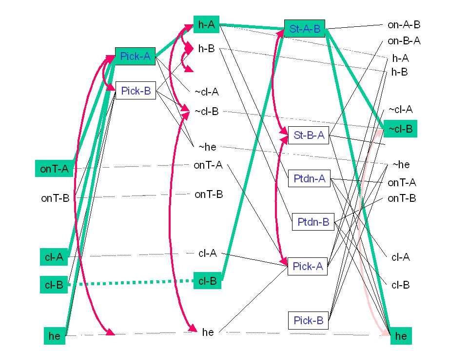
51. onT-A onT-B cl-A cl-B he Pick-A Pick-B onT-A onT-B cl-A cl-B he h-A h-B ~cl-A ~cl-B ~he St-A-B St-B-A Ptdn-A Ptdn-B Pick-A onT-A onT-B cl-A cl-B he h-A h-B ~cl-A ~cl-B ~he on-A-B on-B-A Pick-B Relaxed plan for our blocks example

52. Progression Regression How do we use reachability heuristics for regression?

53. Planning Graphs for heuristics  Construct planning graph(s) at each search node  Extract relaxed plan to achieve goal for heuristic p5 q5 r5 p6 o pq o pr o 56 p5p5 pqr56pqr56 o pq o pr o 56 pqrst567pqrst567 o ps o qt o 67 q5q5 qtr56qtr56 o qt o qr o 56 qtrsp567qtrsp567 o qs o tp o 67 r5r5 rqp56rqp56 o rq o rp o 56 rqpst567rqpst567 o rs o qt o 67 p6p6 pqr67pqr67 o pq o pr o 67 pqrst678pqrst678 o ps o qt o 78 1 3 4 1 3 o 12 o 34 2 1 3 4 5 o 12 o 34 o 23 o 45 2 3 4 5 3 5 o 34 o 56 3 4 5 o 34 o 45 o 56 66 7 o 67 1 5 1 5 o 12 o 56 2 1 3 5 o 12 o 23 o 56 2 66 7 o 67 G oGoG G oGoG G oGoG G oGoG G oGoG 1 3 3 5 1 5 h( )=5

54. h-sum; h-lev; h-relax H-lev is lower than or equal to h-relax H-ind is larger than or equal to H-lev H-lev is admissible H-relax is not admissible unless you find optimal relaxed plan –Which is NP-Hard..

55. PGs for reducing actions If you just use the action instances at the final action level of a leveled PG, then you are guaranteed to preserve completeness –Reason: Any action that can be done in a state that is even possibly reachable from init state is in that last level –Cuts down branching factor significantly –Sometimes, you take more risky gambles: If you are considering the goals {p,q,r,s}, just look at the actions that appear in the level preceding the first level where {p,q,r,s} appear for the first time without Mutex.

56. Negative Interactions To better account for -ve interactions, we need to start looking into feasibility of subsets of literals actually being true together in a proposition level. Specifically,in each proposition level, we want to mark not just which individual literals are feasible, –but also which pairs, which triples, which quadruples, and which n-tuples are feasible. (It is quite possible that two literals are independently feasible in level k, but not feasible together in that level) The idea then is to say that the cost of a set of S literals is the index of the first level of the planning graph, where no subset of S is marked infeasible The full scale mark-up is very costly, and makes the cost of planning graph construction equal the cost of enumerating the full progres sion search tree. –Since we only want estimates, it is okay if talk of feasibility of upto k-tuples For the special case of feasibility of k=2 (2-sized subsets), there are some very efficient marking and propagation procedures. –This is the idea of marking and propagating mutual exclusion relations.

57. Don’t look at curved lines for now… Have(cake) ~eaten(cake) ~Have(cake) eaten(cake) Eat No-op Have(cake) eaten(cake) bake ~Have(cake) eaten(cake) Have(cake) ~eaten(cake) Eat No-op Have(cake) ~eaten(cake) Graph has leveled off, when the prop list has not changed from the previous iteration The note that the graph has leveled off now since the last two Prop lists are the same (we could actually have stopped at the Previous level since we already have all possible literals by step 2)

58. Level-off definition? When neither propositions nor mutexes change between levels

59. Rule 1. Two actions a1 and a2 are mutex if (a)both of the actions are non-noop actions or (b) a1 is any action supporting P, and a2 either needs ~P, or gives ~P. (c) some precondition of a1 is marked mutex with some precondition of a2 Rule 2. Two propositions P1 and P2 are marked mutex if all actions supporting P1 are pair-wise mutex with all actions supporting P2. Mutex Propagation Rules Serial graph interferene Competing needs This one is not listed in the text

60. onT-A onT-B cl-A cl-B he Pick-A Pick-B onT-A onT-B cl-A cl-B he h-A h-B ~cl-A ~cl-B ~he

61. onT-A onT-B cl-A cl-B he Pick-A Pick-B onT-A onT-B cl-A cl-B he h-A h-B ~cl-A ~cl-B ~he St-A-B St-B-A Ptdn-A Ptdn-B Pick-A onT-A onT-B cl-A cl-B he h-A h-B ~cl-A ~cl-B ~he on-A-B on-B-A Pick-B

62. Level-based heuristics on planning graph with mutex relations h lev ({p 1, …p n })= The index of the first level of the PG where p 1, …p n appear together and no pair of them are marked mutex. (If there is no such level, then h lev is set to l+1 if the PG is expanded to l levels, and to infinity, if it has been expanded until it leveled off) We now modify the h lev heuristic as follows This heuristic is admissible. With this heuristic, we have a much better handle on both +ve and -ve interactions. In our example, this heuristic gives the following reasonable costs: h({~he, cl-A}) = 1 h({~cl-B,he}) = 2 h({he, h-A}) = infinity (because they will be marked mutex even in the final level of the leveled PG) Works very well in practice H({have(cake),eaten(cake)}) = 2

63. How about having a relaxed plan on PGs with Mutexes? We had seen that extracting relaxed plans lead to heuristics that are better than “level” heuristics Now that we have mutexes, we generalized level heuristics to take mutexes into account But how about a generalization for relaxed plans? –Unfortunately, once you have mutexes, even finding a feasible plan (subgraph) from the PG is NP-hard We will have to backtrack over assignments of actions to propositions to find sets of actions that are not conflicting –In fact, “plan extraction” on a PG with mutexes basically leads to actual (i.e., non-relaxed) plans. This is what Graphplan does (see next) –(As for Heuristics, the usual idea is to take the relaxed plan ignoring mutexes, and then add a penalty of some sort to take negative interactions into account. See adjusted sum heuristics)

64. How lazy can we be in marking mutexes? We noticed that h lev is already admissible even without taking negative interactions into account If we mark mutexes, then h lev can only become more informed –So, being lazy about marking mutexes cannot affect admissibility Unless of course we are using the planning graph to extract sound plans directly. –In this latter case, we must at least mark all statically interfering actions mutex »Any additional mutexes we mark by propagation only improve the speed of the search (but the improvement is TREMENDOUS) –However, being over-eager about marking mutexes (i.e., marking non-mutex actions mutex) does lead to loss of admissibility

65. PGs can be used as a basis for finding plans directly If there exists a k-length plan, it will be a subgraph of the k-length planning graph. (see the highlighted subgraph of the PG for our example problem)

66. Finding the subgraphs that correspond to valid solutions.. --Can use specialized graph travesal techniques --start from the end, put the vertices corresponding to goals in. --if they are mutex, no solution --else, put at least one of the supports of those goals in --Make sure that the supports are not mutex --If they are mutex, backtrack and choose other set of supports. {No backtracking if we have no mutexes; basis for “relaxed plans”} --At the next level subgoal on the preconds of the support actions we chose. --The recursion ends at init level --Consider extracting the plan from the PG directly -- This search can also be cast as a CSP Variables: literals in proposition lists Values: actions supporting them Constraints: Mutex and Activation The idea behind Graphplan

68. Backward search in Graphplan P1P1 P2P2 P3P3 P4P4 P5P5 P6P6 I1I1 I2I2 I3I3 X X X P1P1 P2P2 P3P3 P4P4 P5P5 P6P6 A5A5 A6A6 A7A7 A8A8 A9A9 A 10 A 11 G1G1 G2G2 G3G3 G4G4 A1A1 A2A2 A3A3 A4A4 P6P6 P1P1 Animated

69. The Story Behind Memos… Memos essentially tell us that a particular set S of conditions cannot be achieved at a particular level k in the PG. –We may as well remember this information— so in case we wind up subgoaling on any set S’ of conditions, where S’ is a superset of S, at that level, you can immediately declare failure “Nogood” learning—Storage/matching cost vs. benefit of reduced search.. Generally in our favor But, just because a set S={C1….C100} cannot be achieved together doesn’t necessarily mean that the reason for the failure has got to do with ALL those 100 conditions. Some of them may be innocent bystanders. –Suppose we can “explain” the failure as being caused by the set U which is a subset of S (say U={C45,C97})—then U is more powerful in pruning later failures –Idea called “Explanation based Learning” Improves Graphplan performance significantly…. [Rao, IJCAI-99; JAIR 2000]

70. Some observations about the structure of the PG 1. If an action a is present in level l, it will be present in all subsequent levels. 2. If a literal p is present in level l, it will be present in all subsequent levels. 3. If two literals p,q are not mutex in level l, they will never be mutex in subsequent levels --Mutex relations relax monotonically as we grow PG 1,2,3 imply that a PG can be represented efficiently in a bi-level structure: One level for propositions and one level for actions. For each proposition/action, we just track the first time instant they got into the PG. For mutex relations we track the first time instant they went away. 4.PG doesn’t have to be grown to level-off to be useful for computing heuristics 5.PG can be used to decide which actions are worth considering in the search

71. Distance of a Set of Literals SumSet-Level Partition-kAdjusted SumCombo Set-Level with memos h(S) =  p  S lev({p}) h(S) = lev(S) Admissible  lev(p) : index of the first level at which p comes into the planning graph  lev(S): index of the first level where all props in S appear non-mutexed.  If there is no such level, then If the graph is grown to level off, then  Else k+1 (k is the current length of the graph)

72. Use of PG in Progression vs Regression Progression –Need to compute a PG for each child state As many PGs as there are leaf nodes! Lot higher cost for heuristic computation –Can try exploiting overlap between different PGs –However, the states in progression are consistent.. So, handling negative interactions is not that important Overall, the PG gives a better guidance even without mutexes Regression –Need to compute PG only once for the given initial state. Much lower cost in computing the heuristic –However states in regression are “partial states” and can thus be inconsistent So, taking negative interactions into account using mutex is important –Costlier PG construction Overall, PG’s guidance is not as good unless higher order mutexes are also taken into account Historically, the heuristic was first used with progression planners. Then they used it with regression planners. Then they found progression planners do better. Then they found that combining them is even better. Remember the Altimeter metaphor..

73.  Distance heuristics to estimate cost of partially ordered plans (and to select flaws)  If we ignore negative interactions, then the set of open conditions can be seen as a regression state  Mutexes used to detect indirect conflicts in partial plans  A step threatens a link if there is a mutex between the link condition and the steps’ effect or precondition  Post disjunctive precedences and use propagation to simplify PG Heuristics for Partial Order Planning

75. What if actions have non-uniform costs?

76. Challenges in Cost Propagation