1. Eigenvalues and eigenvectors
Equilibrium
Population increase
Deaths
Births t
Population increase = Births – deaths
If the population is age structured and contains k age classes we get
N: population size
b: birthrate
d: deathrate
The numbers of surviving individuals from class i to class j are given by
The net reproduction rate R = (1+bt-dt)

2. Leslie matrix
Assume you have a population of organisms that is age structured.
Let fX denote the fecundity (rate of reproduction) at age class x.
Let sx denote the fraction of individuals that survives to the next age class x+1 (survival rates).
Let nx denote the number of individuals at age class x
We can denote this assumptions in a matrix model called the Leslie model. We have w-1 age classes, w is the maximum age of an individual.
L is a square matrix.
Numbers per age class at time t=1 are the dot product of the Leslie matrix with the abundance vector N at time t

3. v v v The sum of all fecundities gives the number of newborns
n0s0 gives the number of individuals in the first age class v
Nw-1sw-2 gives the number of individuals in the last class v
The Leslie model is a linear approach.
It assumes stable fecundity and mortality rates
The effect pof the initial age composition disappears over time
Age composition approaches an equilibrium although the whole population might go extinct.
Population growth or decline is often exponential

4. At the long run the population dies out.
An example
Important properties:
Eventually all age classes grow or shrink at the same rate
Initial growth depends on the age structure
Early reproduction contributes more to population growth than late reproduction
At the long run the population dies out.
Reproduction rates are too low to counterbalance the high mortality rates

5. Leslie matrix
Does the Leslie approach predict a stationary point where population abundances doesn’t change any more?
We’re looking for a vector that doesn’t change direction when multiplied with the Leslie matrix.
This vector is called the eigenvector U of the matrix.
Eigenvectors are only defined for square matrices.
I: identity matrix

6. The insulin – glycogen system
At high blood glucose levels insulin stimulates glycogen synthesis and inhibits glycogen breakdown.
The change in glycogen concentration can be modelled by the sum of constant production and concentration dependent breakdown
At equilibrium we have
The vector {-f,g} is the eigenvector of the dispersion matrix and gives the stationary point.
The value -1 is called the eigenvalue of this system.

7. How to transform vector A into vector B? Y
Multiplication of a vector with a square matrix defines a new vector that points to a different direction.
The matrix defines a transformation in space B A
The vectors that don’t change during transformation are the eigenvectors. X Y
In general we define B
U is the eigenvector and l the eigenvalue of the square matrix X A X
Image transformation
X contains all the information necesssary to transform the image

8. The basic equation
The matrices A and L have the same properties. We have diagonalized the matrix A.
We have reduced the information contained in A into a characteristic value l, the eigenvalue.

9. A nxn matrix has n eigenvalues and n eigenvectors
Symmetric matrices and their transposes have identical eigenvectors and eigenvalues
Eigenvectors of symmetric matrices are orthogonal.

10. How to calculate eigenvectors and eigenvalues?
The equation is either zero for the trivial case u=0 or if [A-lI] =0

11. The general solutions of 2x2 matrices
Distance matrix
Dispersion matrix

12. This system is indeterminate
Matrix reduction

13. Characteristic polynomial
Higher order matrices
Characteristic polynomial
Eigenvalues and eigenvectors can only be computed analytically to the fourth power of m.
Higher order matrices need numerical solutions

14. The power method to find the largest eigenvalue.
The power method is an interative process that starts from an initial guess of the eigenvector to approximate the eigenvalue
Let the first component u11 of u1 being 1.
Rescale u1 to become 1 for the first component. This gives a second guess for l.
Repeat this procedure until the difference ln+1 – ln is less than a predefined number e.
Having the eigenvalues thew eigenvectors come immediately from solving the linear system
using matrix reduction

16. Some properties of eigenvectors
If L is the diagonal matrix of eigenvalues:
The eigenvectors of symmetric matrices are orthogonal
The product of all eigenvalues equals the determinant of a matrix.
Eigenvectors do not change after a matrix is multiplied by a scalar k. Eigenvalues are also multiplied by k.
The determinant is zero if at least one of the eigenvalues is zero.
In this case the matrix is singular.
If A is trianagular or diagonal the eigenvalues of A are the diagonal entries of A.

17. Page Rank In large webs (1-d)/N is very small
A standard eigenvector problem
The requested raking is simply contained in the largest eigenvector of P.

18. A B C D

19. The data points of the new system are close to the new x-axis
The data points of the new system are close to the new x-axis. The variance within the new system is much smaller.
Principal axes u2 u1 u1 u2
Principal axes define the longer and shorter radius of an oval around the scatter of data points.
The quotient of longer to short principal axes measure how close the data points are associated (similar to the coefficient of correlation).
The principal axes span a new Cartesian system .
Principal axes are orthogonal.

20. Major axis regression
The largest major axis defines a regression line through the data points {xi,yi}. u1
The major axis is identical with the largest eigenvector of the associated covariance matrix.
The length of the axes are given by the eigenvalues.
The eigenvalues measure therefore the association between a and y. u2
The first principal axis is given by the largest eigenvalue
Major axis regression minimizes the Euclidean distances of the data points to the regression line.

21. The relationship between ordinary least square (OLS) and major axis (MAR) regression

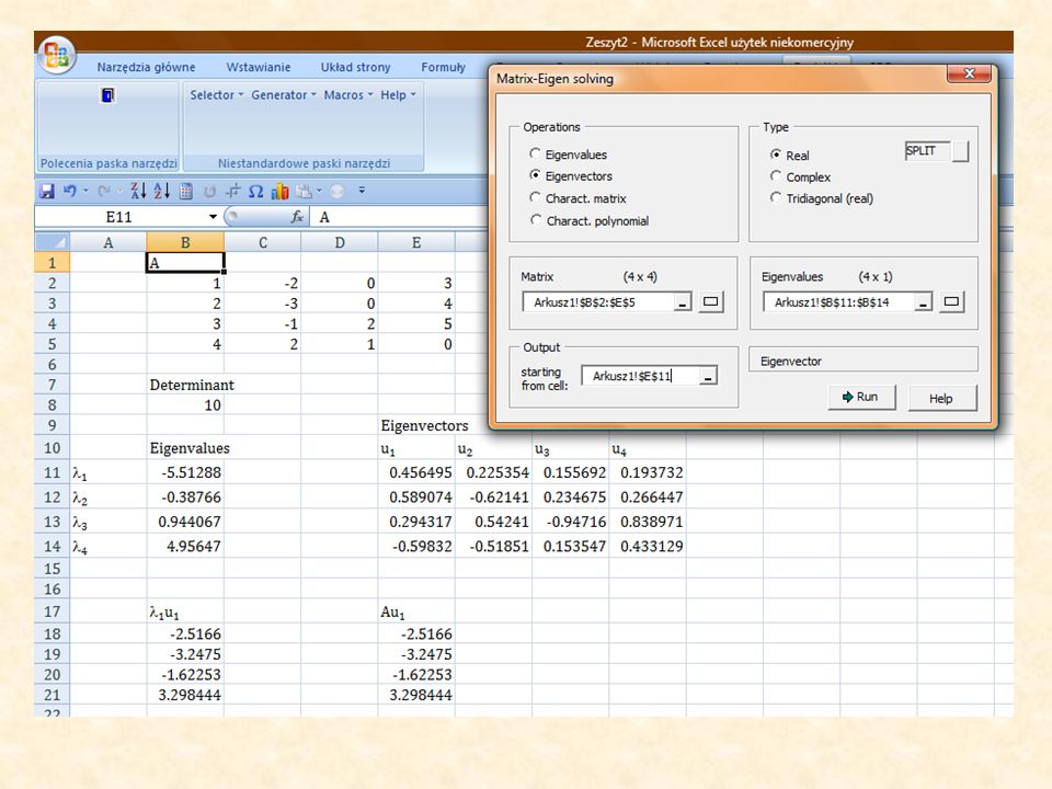
22. Going Excel

23. Ordinary least squares regression (OLS) Major axis regression (MAR)
Errors in the x and y variables cause OLS regression to predict lower slopes. Major axis regression is closer to the correxct slope.
Ordinary least squares regression (OLS)
Major axis regression (MAR)
The MAR slope is always steeper than the OLS slope.
If both variables have error terms MAR should be preferred.

24. MAR is not stable after rescaling of only one of the variables
Days/360
MAR should not be used for comparing slopes if variables have different dimensions and were measured in different units, because the slope depends on the way of measurement.
If both variables are rescaled in the same manner (by the same factor) this problem doesn’t appear.
OLS regression retains the correct scaling factor, MAR does not.

25. A simple way to take the power of a square matrix
Scaling a matrix
A simple way to take the power of a square matrix

26. The variance and covariance of data according to the principal axisy
(x;y)
The vector of data points in the new system comes from the transformation according to the principal axes u1 u2 x
Eigenvectors are normalized to the length of one
The eigenvectors are orthogonal
The variance of variable k in the new system is equal to the eigenvalue of the kth principal axis.
The covariance of variables j and k in the new system is zero. The new variables are independent.