1. Electronic structure of correlated electron systems George Sawatzky UBC Lecture 4 2011

2. Back to the simplest possible model for strong correlation A Hubbard model for the hydrogen molecule

3. H2+ molecule for only 1 electron Obviously there is no correlation Solutions are a bonding and antibonding orbital with a separation of 2t Things change when we go to two electrons

4. i.E two electrons on one site. These should be high energy states because of the coulomb interaction U. These high polarity states should be projected out for large U H2 model in strong correlation One electron molecular orbital theory H atoms A and B Splitting =2t

5. Two hydrogen atoms each with one electron Triplet state Singlet state Heitler London Model For t=0 Now add finite t with configuration interaction (CI)

6. Heitler London limit + CI For U>>t Singlet is lower in energy than triplet by Low energy scale excitations are spin only excitations

7. The influence of U As we noted before U reduces the polarity fluctuations U drives the system to be magnetic for open shell systems U results in low energy scale magnetic degrees of freedom

8. The Hubbard model is not exactly solvable except in 1 D but even then the spectral functions are difficult to extract Lieb and Wu PRL 20, 1445, (1968)

9. 1D Hubbard exact and not so exact solutions Lieb and Wu PRL 20, 1445 (1968) For half filled s band the band gap t=1 Gutzwiller approximation ( any dimension) Variational wave function with weight of doubly occupied sites decreasing as U/w increases. η =variational parameter v= average no of doubly occupied sites Q(v) =band narrowing, W=2Zt; Z=nnn Physical Review 137: A1726.

10. Thesis van den Brink Groningen

11. A bit more about simple models and some peculiar properties in 1 and 2 dimensions of the simple models

12. Magnetic excitations in ½ filled Hubbard or Mott insulators Magnon S=1 Two spinons each with s=1/2 Spinons propagate via J S i + S - 1+1 Magnons and spinons in 1D Neel antiferromagnet Once the spinons have moved through the central region looks like all the spins have reversed

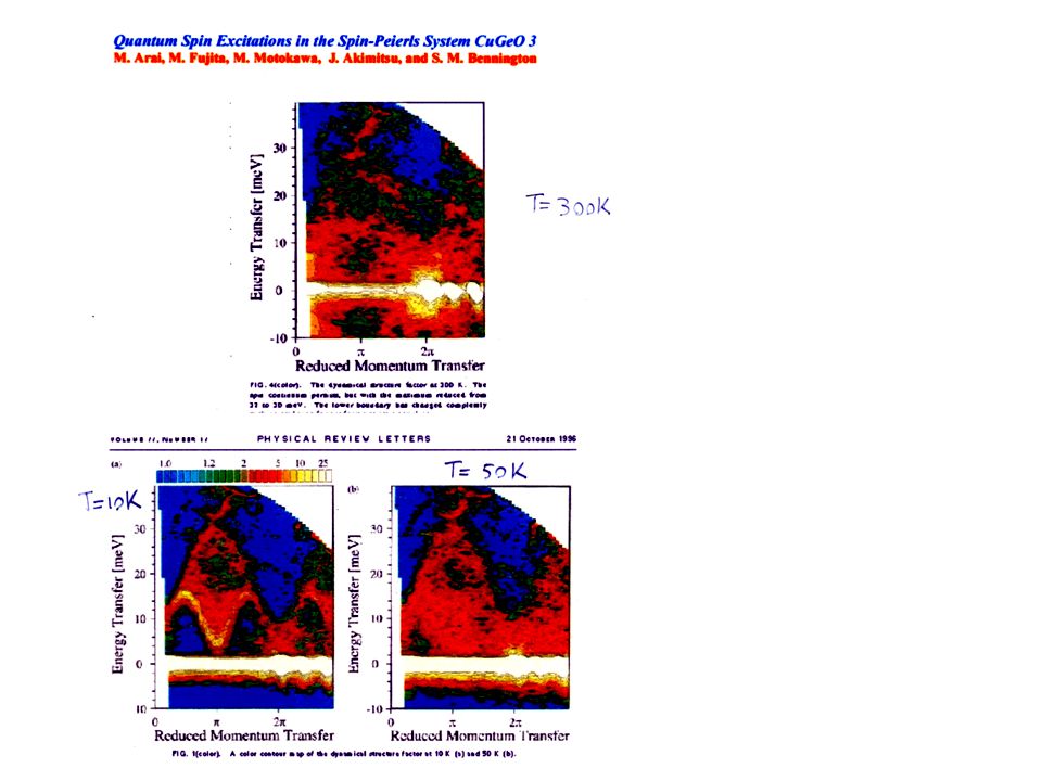
13. Inelastic Neutron scattering

15. Heisenberg In two and three dimensions In higher dimensions the magnetic excitations are much more like conventional magnons although a lesson also there can be learned from the 1D case. In 1D it has been known theoretically since 1983 that the actual magnetic excitations are spinons and not magnons. Neutron inelastic scattering also in 1D may look somewhat like magnons but it was only after one looked carefully at smaller structures and the “ background” that one could recognize the spinon character of the excitations. Tennant et al PRB532, 13358 (1995) Although it seems difficult to define spinons in 2 and 3D there will be incoherent contributions to the magnon excitations since magnons like other quasi particles will be dressed. Haldane PRL 50 1153 (1983) and ibid 93A, 464 1983

16. Vladimir Hinkov a Max Planck /UBC QMI visiting professor will give a lecture on Neutron scattering in March in which some of these aspects will be addressed

17. |Doped systems” i.e.Less than ½ filled Hubbard S band J t Consider U>>t and the t,J model Sums are for j a nearest neighbor to i Avoids double occupancy Goes to a spin only Heisenberg Hamiltonian for half filling Although this Hamiltonian looks plausible for U>>t I do not know of any real proof of the transformation from Hubbard to t,J There also is no exact solution of the tJ model The tJ model is one of the most used models in attempts To describe the high temperature superconducting cuprates

18. For J very small we might think of a spinless Fermion model in which a single Slater Determinant of single particle Bloch states would be eigenfunctions of H and at the same time the single particles would avoid being on the same site because they are Fermions. In this model all signs of magnetism would disappear. It however takes care of double occupancy and still remains otherwise single particle like. In this Spinless Fermion model We see that each Fermion indeed blocks two states of the initial Hubbard model

19. Spin charge separation in 1D Antiphase Domain wall Now the charge is free to move so we have two free particles a Spinon and a holon!! A single electron removed from a half filled large U antiferromagnet Hole created at site zero Hole hops to the right via t 2 nd and 3 rd spin to the left exchange Spinon moves to the left viaJ S i - S + i-1 Spinon is gone leaving the hole at an antiferromagnetic antiphase domain wall and now free to move

20. B.J. Kim, H. Koh, E. Rotenberg, S.-J. Oh, H. Eisaki, N. Motoyama, S. Uchida, T. Tohyama, S. Maekawa, Z.-X. Shen, and C. Kim, Nature Physics 2, 397 (2006)., " Distinct spinon and holon dispersions in photoemission spectral functions from one-dimensional SrCuO 2," Angular resolved photelectron spectroscopy measurements Spinon Holon

21. Spinon and Holon Dispersion The spinon hops two sites at a time so the period is basically 2a with a the lattice constant. The effective hoping integral is J (in actual fact it is J π/2) since this flips the appropriate spins to move the spinon. The holon moves with a hoping integral t. The spinons are fermions and the spinon band is half full to start with πJ|sin(k−π/2)|/2 (|k| ≤ π/2) and the holon branch with 2t cos(k±π/2), respectively The above is a formal theory of spinons in which they are considered as spin ½ particles added to the system qhen we remove an electron and with the antiferromagnetic ground state being a Fermi gas of spinons with the the Fermi level corresponding to half filling. A poor mans way of describing the the spin change separation and spinon holon dispersion is as drawn above. Here the spinon lives on a lattice of period 2a and hops with hoping integral J and the holon lives on a lattice of lattice constant a and hops with a hoping integral t. This gives the same dispersion as above except for the factor of pi/2 for the spinon hopin.

22. The propagation of a hole in a two D antiferromagnetic background Starting position of A hole Final position of A hole A hole moves by hoping an electron into it from a neighboring site conserving the spin. This movement leaves a chain of wrongly oriented spins behind at a large energy cost. Looks like a self confining potential is created. How can this be repaired?

23. Try to repair with either the or with two holes moving together the second hole following the first can repair the damage of the first if they are on neighboring sites creating an effective attractive interaction. The pair is now free to move!! Also less exchange bonds are broken if they are on nn sites.

24. In A NEEL ANTIFERROMAGNET AS DRAWN ABOVE THE SPINS ARE UP OR DOWN AND QUANTUM FLUCTUATIONS ARE ASSUMED TO BE ABSENT. THIS IS FAR FROM REALITY FOR A 1D SPIN ½ SYSTEM AND ALSO TO A LESSER DEGREE FOR A 2D SYSTEM WITH SPINS OF ½. In 1D long range order cannot exist and in 2D antiferromagnetic long range order can only exist at T=0. However both in 1D and 2D the antiferromagnetic correlations exist over a long range increasing in length as T decreases. Tn of about 300K in the high tc superconducting parent compounds is not representative of the large J=140meV or about 1500K but is representative of the small interplaner coupling J’ times the spin spin correlation length build up in the planes due to J. A few remarks about magnetic ordering

25. Singlet liquid RVB wins over long range order for Z <3. i.e. in 1D and perhaps perhaps in hole doped 2D system Resonant valence bond vs Neel Energy of Classical antiferromagnetic Neel state N = no of sites, Z= number of nearest neighbors, and J = exchange between nearest neighbors Energy of a nearest neighbor RVB singlet liquid state Energy of a singlet is 3J/4

26. Some interesting two particle problems Recall we have an exact solution so have a look at some simple model molecules such as atoms in a triangle or square etc for U>> t and for two electrons or two holes and check for the singlet triplet splitting.

27. For U >>>t the two particles never see each other so is there a singlet triplet splitting?

28. Example of two particles in U=  limit t t tt 11 2221 Triplet Singlet “+” for singlet; “-” for triplet Energy level diagram for holes (t>0) -2t -t t 2t Triplet Singlet

29. Strong singlet triplet splitting as a result of symmetry Singlet is lowest in energy for t<0 or for electrons Triplet is lowest for t>0 or for holes The energy splitting is determined by t the hoping integral not by some coulomb or exchange interaction Potential for new magnetic materials without magnetic elements like the 3d transition metals of rare earths

30. Similar is some sense to the 1D case it is proposed that for a 2D system with finite doping one has rivers of charge separating anti-phase antiferromagnetic domain walls. Also called electronic nematic ordering. Charges can now fluctuate from left to right without costing exchange energy. Anisimov, Zaanen,Andersen, Kivelson,Emery-----

31. Coulomb interactions in solids How large is U ? How are interactions screened in solids?

32. Do we need screening at all? In the beginning we showed that we know the exact Hamiltonian and the exact equation we have to solve to understand the electronic structure of solids Indeed if we could do this then no need for screening and effective parameters Because we can’t solve the above we use models and it is in those models where not all interactions and states are included. This requires us to include whatever is not included in a “renormalization “ of the parameters in the models.

33. For a Hubbard model for example We have to include the effects of all the longer range coulomb interactions in an effective “U” and hoping integrals t We have to include the effects of all the other states not included explicitly in H on U and t Perhaps we have to add some longer range interactions like V=nearest neighbor coulomb and longer range hoping than nearest neighbor

34. How to include longer range and off diagonal interactions Screening??? But what about the reduction of short range interactions?

35. Start with the conventional assumption of a uniform polarizable medium.

36. From Auger spectroscopy we know U is strongly reduced in the solid How can U be reduced in the solid? Surely we cannot use U=U0/Є with Є= dielectric constant? After all no “screening “ charge can get between the two electrons on the same atom. We have to go back to the original definition of U in terms of ionization potential and electron affinity. Lets first review conventional screening valid for long range interactions.

37. Homogeneous Maxwell Equations  (r,r ’ ) —>  (r – r ’ ) —>  (q) Ok if polarizability is uniform In most correlated electron systems and molecular solids the polarizability is actually Very NONUNIFORM

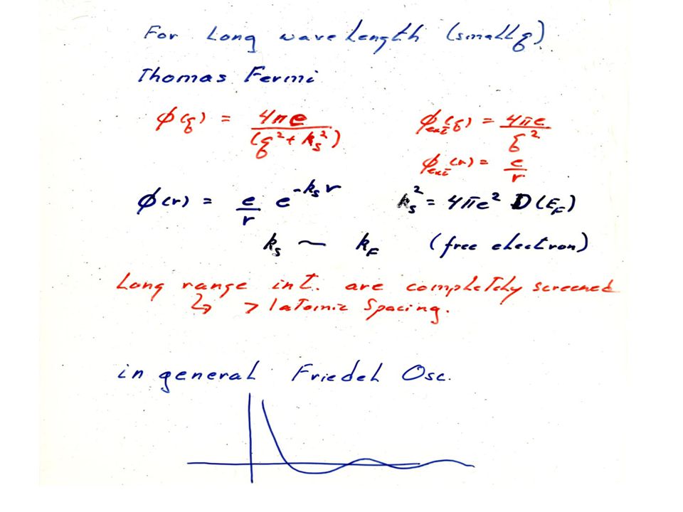
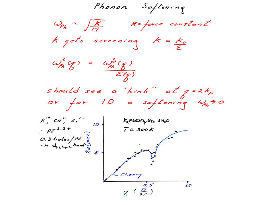
38. Review uniform polarizability approach Maxwell =screened potential Poisson Free electron gas in one,two and three dimensions Response to a static (external like an impurity ) potential Screening potential Phonon softening and Giant Kohn anomaly

39. Electron density =n(r) = Take a potential of the form Free electron wave function and energy i.e. φ(r) =const

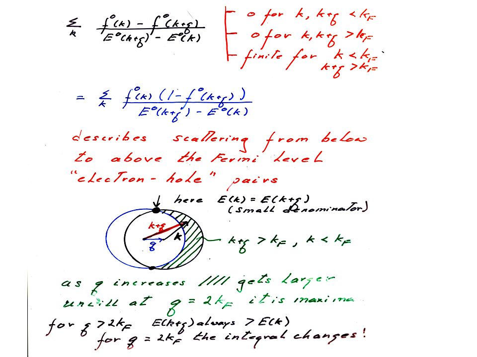
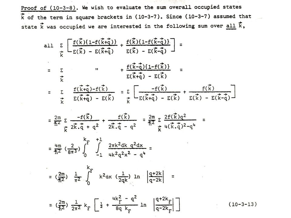
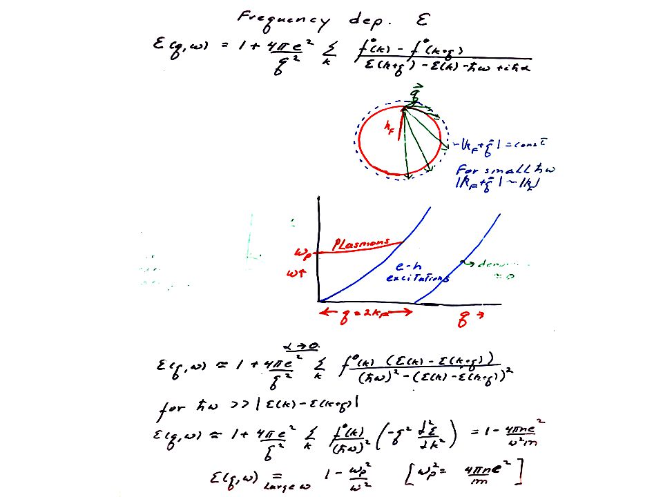
40. Perturbation theory approach f’s are the occupation numbers and the sum is over the possible excitations from below to above the Fermi energy. Use Poisson to get the induced potential

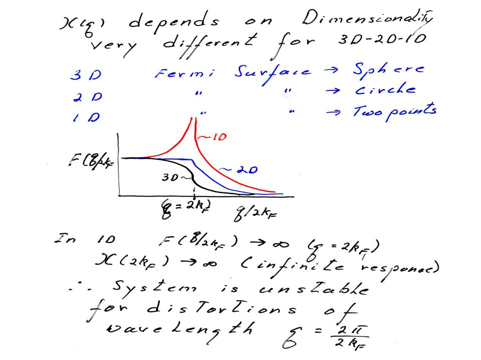
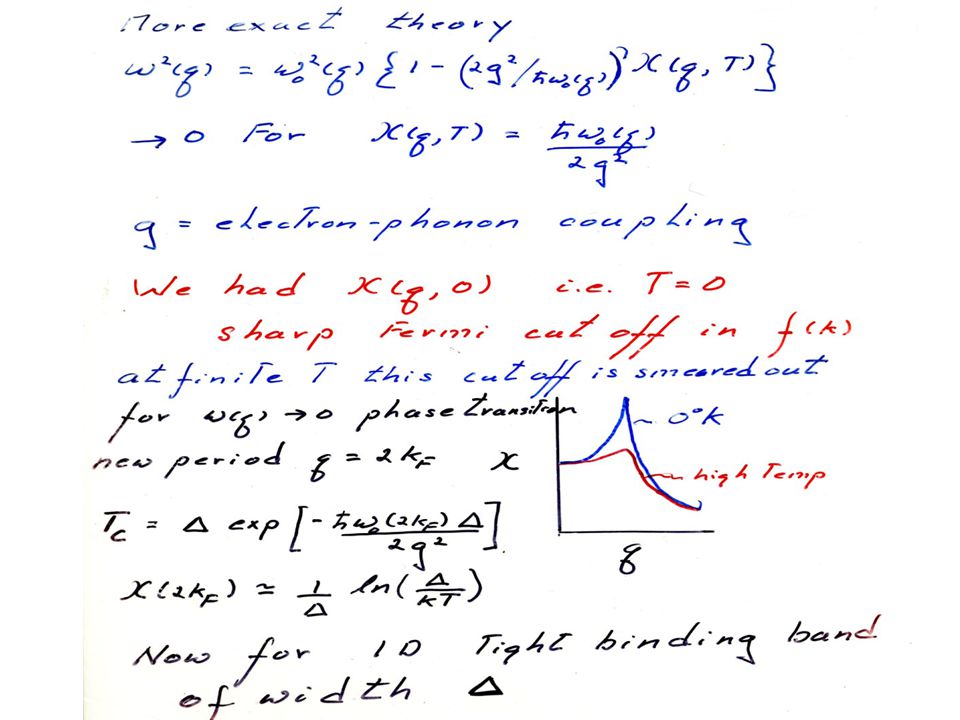
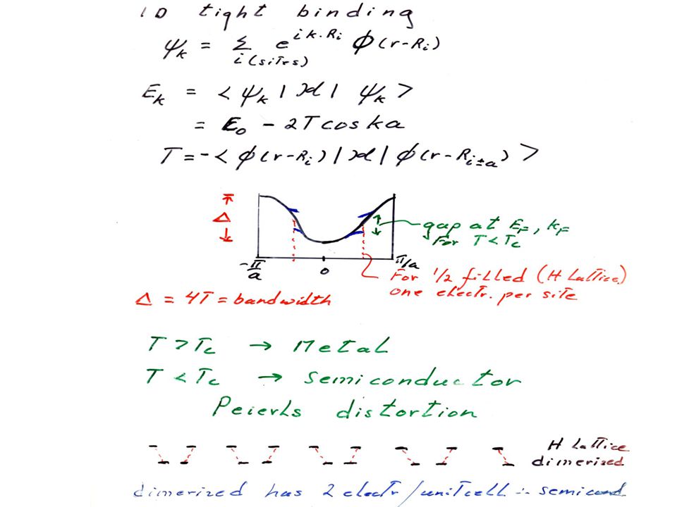
47. Consequences of the anomalous 2kf behaviour of the Lindhard function at Friedel charge density Oscillations-RKKY Ruderman-Kittel-Kasuya-Yoshida long range exchange interactions in metals Giant Kohn Anomaly---phonon softening for q=2kf Fermi surface nesting in 2D Semiconductor metal transition –Peierls transition both charge and spin Peierls