Download presentation
Presentation is loading. Please wait.

1
Open source tools for computational biology
Craig A. Stewart, Richard Repasky, and Andrew Arenson Indiana University SC2004 Tutorial S06 7 November 2004

2
License terms Please cite as: Stewart, C.A., R. Repasky, A. Arenson Open source tools for computational biology. Tutorial presented at SC2004, 6-12 Nov 2004, Pittsburgh, PA. Some figures are shown here taken from web, under an interpretation of fair use that seemed reasonable at the time and within reasonable readings of copyright interpretations. Such diagrams are indicated here with a source url. In several cases these web sites are no longer available, so the diagrams are included here for historical value. Except where otherwise noted, by inclusion of a source url or some other note, the contents of this presentation are © by the Trustees of Indiana University. This content is released under the Creative Commons Attribution 3.0 Unported license ( This license includes the following terms: You are free to share – to copy, distribute and transmit the work and to remix – to adapt the work under the following conditions: attribution – you must attribute the work in the manner specified by the author or licensor (but not in any way that suggests that they endorse you or your use of the work). For any reuse or distribution, you must make clear to others the license terms of this work.
. For any reuse or distribution, you must make clear to others the license terms of this work.")
3
Planned schedule for the day
8:30-8:40 Introduction and objectives 8:40-9:00 An introduction to the biological basis and biological data sources 9:00-10:00 Pattern matching 10:00-10:30 Break 10:30-11:15 Hands-on problem session 11:15-12:00 Multiple sequence alignment 12:00-13:30 Lunch 13:30-14:15 Microarray data analysis 14:15-15:00 RNA and Protein Structure 15:00-15:30 Break 15:30-16:15 Problem session II 16:15-17:00 Systems Biology

4
Table of Contents Class Plan and Objectives 4
A rapid introduction to key elements of biology 12 Bioinformatics data sources Similarity matching Multiple sequence alignment Microarray data analysis RNA and Protein Structure 119 Systems Biology Acknowledgements & references 155 Appendix 1: DNA sequencing 157 Appendix 2: Phylogenetics 161 Appendix 3: Grand challenge problems 169 Note: Slides with the Indiana University wordmark in the bottom left corner were generated at Indiana University, with images sometimes from other sources. In such cases the url for the source of the image is indicated on the slide. Slides with a plain white background have been graciously provided by someone outside IU, and sources are attributed on such slides. Appendices cover material of potential interest to the attendees, but will not be covered in class

5
Class Plan & Objectives
Class Plan & Strategy Materials focus on open source software (generally not the presenters own work) One critical application will be covered in great depth, and several others will be reviewed Objectives. At the end of the class, participants should: understand enough biology to understand key computational biology problems, and be familiar with some strategies for collaborating with biologists and biomedical scientists be conversant with key open source applications in computational biology and bioinformatics, and current problems in these areas Be ready to download some code and start making it better!
 One critical application will be covered in great depth, and several others will be reviewed. Objectives. At the end of the class, participants should: understand enough biology to understand key computational biology problems, and be familiar with some strategies for collaborating with biologists and biomedical scientists. be conversant with key open source applications in computational biology and bioinformatics, and current problems in these areas. Be ready to download some code and start making it better!")
6
Motivation The “-omics” trend
Finding press pieces about huge computing problems is easy How many bio codes really scale to hundreds of processors? What are the coming high performance needs of biologists? Importance of computational biology and bioinformatics to the HPC community The challenges and promise are real Successes and failures so far Successes: Protein structure, Genome assembly, Surgical assistance, Phylogenetics Mismatched priorities: Ab initio protein folding Not yet successful: Drug discovery

7
What has changed recently?
Bioinformatics not new Protein structure Phylogenetics What is new is high-throughput sequencing: Lots more data The possibility of going from a knowledge of the DNA sequence to an understanding of diseases and health

8
Genome Projects Timeline
First virus (SV40) sequenced (5224 base pairs) DOE announces Human Genome Initiative First complete map of all human chromosomes First living organism sequenced (H. influenzae) 2 Mb Yeast (S. cerevisiae) - 12 Mb Intestinal bacterium (E. coli) - 5 Mb Nematode worm (C. elegans) Mb Celera announcement; Public effort regroups Human Chromosome 22 – 34 Mb Joint announcement by NHGRI – Celera “As good as it gets” human genome This slide based on slide by Manfred D. Zorn
 sequenced (5224 base pairs) 1986 DOE announces Human Genome Initiative First complete map of all human chromosomes First living organism sequenced (H. influenzae) 2 Mb Yeast (S. cerevisiae) - 12 Mb Intestinal bacterium (E. coli) - 5 Mb Nematode worm (C. elegans) Mb Celera announcement; Public effort regroups Human Chromosome 22 – 34 Mb Joint announcement by NHGRI – Celera As good as it gets human genome. This slide based on slide by Manfred D. Zorn.")
9
Definitions Computational Biology: any use of advanced information technology in the study of biological problems. “Bioinformatics applies the principles of information sciences and technologies to make the vast, diverse and complex life sciences data mnore understandable and useful” (NIH BISTIC Committee grants1.nih.gov/grants/bistic/CompuBioDef.pdf) Genomics – study of genomes and gene function Proteomics – study of proteins and protein function ___omics –
 Genomics – study of genomes and gene function. Proteomics – study of proteins and protein function. ___omics –")
10
Challenges Different types of biological data at different scales
Data of varying quality Much of the underlying biology is not well understood Prior to the availability of high-throughput sequencing, scientists could only study small pieces of the genetic information of any organism. Now the entire genome of several organisms has been completed, but knowing the genome is different than knowing how it works!

11
Comparison of Complexity
Physics & Chemistry 2 elementary particles 4 forces 112 elements When random events occur it is often possible to study average behavior Typically ahistoric (astrophysics an exception) Biology 3B base pairs in humans Min. 30,000 genes in humans ~1.5M species Individual random events important; no law of large numbers Intensely historic, heavily contingent
 Biology. 3B base pairs in humans. Min. 30,000 genes in humans. ~1.5M species. Individual random events important; no law of large numbers. Intensely historic, heavily contingent.")
12
Complexity, Con't Chip design Cells All components known
Device physics for individual components known Itanium has 3 x 10^8 connections and 2 x 10^8 devices Unified basic currency (electrons) Computer program required to understand (e.g. SPICE) Cells Components not known Function of individual components not known # components ~10^13 No unified basic currency Ecell, Karyote, etc. attempting to model cells Computer programs do not yet permit full understanding
 Computer program required to understand (e.g. SPICE) Cells. Components not known. Function of individual components not known. # components ~10^13. No unified basic currency. Ecell, Karyote, etc. attempting to model cells. Computer programs do not yet permit full understanding.")
13
A rapid introduction to key elements of biology

14
Why is it important to know some biology?
Would you study numerical methods without knowing some mathematics? Much current biological knowledge is very specific to particular organisms, genes, or diseases If you just wade into the available data online you can do some very silly things. Anopheles gambiae From mosquito/mtm/index.html Source Library:Centers for Disease Control Photo Credit:Jim Gathany

15
Central dogma of biology
The central dogma of biology is that genes act to create phenotypes through a flow of information form DNA to RNA to proteins, to interactions among proteins (regulatory circuits and metabolic pathways), and ultimately to phenotypes. Collections of individual phenotypes constitute a population (first put forward by Crick in 1958)
, and ultimately to phenotypes. Collections of individual phenotypes constitute a population (first put forward by Crick in 1958)")
16
Cell Structure Eukaryotes Chromosomes linear
Eukaryotes Chromosomes linear Introns, exons, postprocessing Nucleus & nuclear wall Mictochondria and (in plants) Chloroplasts Prokaryotes Chromosome circular Location is everything No nucleus No plastids
 Chloroplasts. Prokaryotes. Chromosome circular. Location is everything. No nucleus. No plastids.")
17
Four (or Five) Bases DNA consists of four nucleotides: Cytosine, Thymine, Adenine, and Guanine. In the double helix, A&T are always bound, and C&G are always bound to each other RNA consists of four nucleotides as well: Cytosine, Uracil, Adenine, and Guanine RNA may loop back on itself but it does not form a double helix

19
Genetic Code Ala Alanine Leu Leucine Arg Arginine Lys Lysine
Asn Asparagine Asp Aspartic acid Cys Cysteine Glu Glutamic acid Gln Glutamine Gly Glycine His Histidine Ile Isoleucine Leu Leucine Lys Lysine Met Methionine Phe Phenylalanine Pro Proline Ser Serine Thr Threonine Trp Tryptophan Tyr Tyrosine Val Valine Original8Hour/Genetics/geneticcode.html

20
Translating DNA to RNA and Transcribing RNA to Proteins
AAAAAGGAGCAAATT DNA 1 4 2 5 3 6 UUUUUCCUCGUUUAA RNA One possible amino acid string Phe Asn Asp Ala

21
Human Chromosomes http://www.ncbi.nlm.nih.gov/Class/MLACourse
/Original8Hour/Genetics/cytogenetic.html Human_Genome/graphics/slides/ elsikaryotype.html

22
Sickle Cell Normal RBC GAG codes for Glutamine disc-Shaped, soft
easily flow through small blood vessels lives for 120 days Sickle RBC GTG codes for Valine sickle-Shaped, hard often get stuck in small blood vessels lives for 20 days or less Malaria vs. Anaemia! ency/imagepages/1223.htm

23
What is a Gene? An inheritable trait associated with a region of DNA that codes for a polypeptide chain or specifies an RNA molecule which in turn has an influence on some characteristic phenotype of the organism. Early views: genes lined up on the chromosome like beads on a string; one gene => one protein Examples of genes: color blindness, sickle-cell anaemia Mendelian genes, Sex-linked genes, Quantitative traits Annotation: Extraction, definition, and interpretation of features on the genome sequence Annotations vs. genes: Many annotations describe features that constitute a gene. Others may not always directly correspond in this way An annotation is what we think… nature may disagree! Inheritance problem with annotations

24
Gene Components Prokaryotes Location is everything
Essentially all of the DNA is transcribed (few mitochondrial diseases) Eukaryotes Non-contiguous pieces of DNA may comprise one gene Start sequence (complicated and long) Stop Codons – end transcription Exons – portions of sequence that are transcribed and used Introns – portions of sequence that are not used Genes and Chromosomes In eukaryotes, an organism has two of each chromosome (in pairs). Among sexually reproducing organisms, one chromosome comes from each parent In “simple Mendelian genes” there are two alleles for each gene – one on each chromosome (e.g. wrinkly)
 Eukaryotes. Non-contiguous pieces of DNA may comprise one gene. Start sequence (complicated and long) Stop Codons – end transcription. Exons – portions of sequence that are transcribed and used. Introns – portions of sequence that are not used. Genes and Chromosomes. In eukaryotes, an organism has two of each chromosome (in pairs). Among sexually reproducing organisms, one chromosome comes from each parent. In simple Mendelian genes there are two alleles for each gene – one on each chromosome (e.g. wrinkly)")
25
Alternate splicing

26
A (very) little about evolutionary genetics
Hardy-Weinberg Law Parents Ww Ww Offspring WW Ww Ww ww Based on this, can you explain why the gene for Sickle Cell Anaemia persists in populations of people in Africa?

27
Population genetics & evolution
Mutations create the raw material for evolution Natural selection and chance affect the frequency with which particular genes or DNA sequences are present in populations Given enough time and enough change, evolution, speciation, and so forth happen Genes can be ‘fixed’ or ‘maintained in an equilibrium’ in a population by chance or through natural selection

28
How do sequences differ?
CGTACCGTTAATAT CGTACCGATAATAT Differences in individual bases Bases may be added to a sequence Bases may be deleted from a sequence CGTACCCCGTAATAT CGTACC . .GTAATAT CGTACCGTTAATAT CGTACCG . . .ATAT

29
Random genetic change “things happen” Molecular clock
theory – ~ 2% change per million years (2 x 10⁻⁹ substitutions per base location per year) Practice – a rule of thumb is different than something like Newton’s 2nd law of motion Random change may often be responsible for speciation – e.g. two populations of birds, separated by a geographic barrier, may at random eventually develop into two different species
 Practice – a rule of thumb is different than something like Newton’s 2nd law of motion. Random change may often be responsible for speciation – e.g. two populations of birds, separated by a geographic barrier, may at random eventually develop into two different species.")
30
Key points (so far) Biological processes are complicated; the historicity and complexity of biological processes and our lack of understanding of many matters makes biology an interesting topic! The fundamental dogma of molecular biology is that genes act to create phenotypes through a flow of information form DNA to RNA to proteins, to interactions among proteins (regulatory circuits and metabolic pathways), and ultimately to phenotypes. Collections of individual phenotypes constitute a population. DNA consists of four base pairs (ATCG). A is always paired with T; C always paired with G. DNA is translated into RNA. RNA consists of four base pairs as well (AUCG). The linear structure of DNA is transcribed into RNA and then into proteins. Proteins have their 3D configuration as the basis for their structure.
, and ultimately to phenotypes. Collections of individual phenotypes constitute a population. DNA consists of four base pairs (ATCG). A is always paired with T; C always paired with G. DNA is translated into RNA. RNA consists of four base pairs as well (AUCG). The linear structure of DNA is transcribed into RNA and then into proteins. Proteins have their 3D configuration as the basis for their structure.")
31
Bioinformatics data sources

32
Bioinformatics Data Sources
There are many Characteristics vary There are many ways to organize view of the biological data A pragmatic approach: Biomedical literature sources Structured vocabularies DNA, RNA, Protein etc. data sources

33
Biomedical literature
Abstracts of biomedical lit. largely available online Text processing itself is an interesting problem U.S. National Library of Medicine – NLM Medline ~12 million references on life sciences/biomedicine. Covers 1966 to present. Citations from over 4,600 journals; most published in English

34
PubMed Standard search tool for Medline Structured Language - Medical Subject Heading ~17,000 Thesaurus Terms, typically used per article in MedLine; 3-4 as major points (indicated with * in PubMed) Annotation done by humans You can save queries
 Annotation done by humans. You can save queries.")
35
Genomic, Proteomic, etc. data sources
A tremendous amount of data is available through public data sources via the Web, ftp, or by other means. To analyze biological data, we first have to get it…. Several ways to organize presentation of material – by site, by type, etc. We will organize by data type. Types of Databases: Chromosomal ( DNA/Genes Protein Biochemistry and metabolic pathways Microarray Web collections

36
Types of genomic data Genomic DNA: DNA sequences, typically complete with coding and non-coding sequences GSS: Genome survey sequence. Single pass sequence read directly from robot. mRNA: an RNA sequence from an mRNA molecule. May or may not cover all of a particular gene cDNA: complement DNA – a DNA sequence generated by conversion of an mRNA sequence EST: Expressed Sequence Tag – short cDNA sequences from studies of cells under particular circumstances. Typically incomplete. SNP – Single Nucleotide Polymorphism

37
DNA databases GenBank. Operated by NCBI (National Center for Biotechnology Information). European Molecular Biology Laboratory – Nucleotide Sequence Database. DNA Database of Japan (DDBJ). All share data daily. Update conflicts avoided by policy. Differences are in “value added” and interfaces
. All share data daily. Update conflicts avoided by policy. Differences are in value added and interfaces.")
39
Data Structures Current
Primary DNA repository data based on ASN.1. Makes possible linkages among many types of biomedical info. The software libraries now often handle XML as well Software toolkits and docs available at Genbank Flat File format FASTA >gi|532319|pir|TVFV2E|TVFV2E envelope protein ELRLRYCAPAGFALLKCNDADYDGFKTNCSNVSVVHCTNLMNTTVTTGLLLNGSYSENRT QIWQKHRTSNDSALILLNKHYNLTVTCKRPGNKTVLPVTIMAGLVFHSQKYNLRLRQAWC

40
Primary vs. Secondary Data sources
Primary data sources: Genetic sequences in NCBI, EMBL, DDJP Protein sequences in PDB Secondary data sources: Inferred protein sequences (what do we know already about issues here?) Curated data sources
 Curated data sources.")
41
Protein Structure NCBI (of course…)
Swiss-Prot/TrEMBL at Note: 125,744 chemically determined vs 861,482 inferred from automated translation of DNA sequences!!!!! Protein Data Base – PDB - one of the first online bioinformatics databases!!!

42
Biochemistry and pathways
ENZYME (part of the ExPASy system) BIND (part of the NCBI system) Pathways PathDB Kegg WIT
 BIND (part of the NCBI system) Pathways. PathDB Kegg WIT")
43
Web Resources - General NCBI http://www.ncbi.nlm.nih.gov/
EBI Biocatalog IUBio Archive

44
Similarity matching

45
Why pattern matching (and what are the problems)
US! and… Bonobo

46
Problems! For proteins, 95% similarity is ~ identical, 80% similarity is a lot. Even less similarity than that needed for DNA Database techniques inadequate – they are too precise! Datasets very large to search Homology Common ancestry Sequence (and usually structure) conservation Homology is inferred rather than measured Identity Objective and well defined Can be quantified easily, but not very useful! Similarity Most common method used, but not as easily defined
 conservation. Homology is inferred rather than measured. Identity. Objective and well defined. Can be quantified easily, but not very useful! Similarity. Most common method used, but not as easily defined.")
47
Alignment An alignment is an arrangement of two sequences opposite one another It shows where they are different and where they are similar We want to find the optimal alignment - the most similarity and the least differences Alignments have two aspects: Quantity: To what degree are the sequences similar (percentage, other scoring method) Quality: Regions of similarity in a given sequence
 Quality: Regions of similarity in a given sequence.")
48
Alignment Methods: dynamic programming Hidden Markov Models Pattern matching Key problem: keeping the calculation time manageable Some alignment packages: BLAST ( FASTA (

49
Scoring Alignments CGTACCGTTAATAT CGTACCG . . .ATAT CGTACCGTTAATAT
GCTAAATTC ++ x x GC AAGTT Matches are good: they get a positive value Mismatches are bad: they get a negative value Gaps are bad: they get a negative value Gap opening penalty Gap extension penalty Score = Matches –Mismatches -∑{gap opening penalty +(length)*gap length penalty} CGTACCGTTAATAT CGTACCG . . .ATAT CGTACCGTTAATAT CGT. C . GTT .ATAT
*gap length penalty} CGTACCGTTAATAT. CGTACCG . . .ATAT. CGTACCGTTAATAT. CGT. C . GTT .ATAT.")
50
Now what? Taking a sequence and simply comparing it against all existing sequences in a database in all possible ways approaches O(N!) if you do it badly enough. Plus it would be silly. So: many algorithms possible Algorithms are in some ways the same, and in some ways different, between DNA and proteins. We’ll start with DNA, and not do things in historical order
 if you do it badly enough. Plus it would be silly. So: many algorithms possible. Algorithms are in some ways the same, and in some ways different, between DNA and proteins. We’ll start with DNA, and not do things in historical order.")
51
Dotter Simple way to get a feel for how sequences compare to each other. Used both with DNA and Protein sequences "A dot-matrix program with dynamic threshold control suited for genomic DNA and protein sequence analysis" Erik L.L. Sonnhammer and Richard Durbin Gene 167(2):GC1-10 (1995) Modular nature of proteins
:GC1-10 (1995) Modular nature of proteins.")
52
Local Alignments with BLAST
Basic Linear Alignment Search Tool We’ll spend a LOT of time with BLAST First a quick demo (hopefully) So, what did we do? BLAST – Basic Linear Alignment Search Tool In particular, BLASTn (for nucleotides) Altschul, S.F., Gish, W., Miller, W., Myers, E.W., and Lipman, D.J Basic Local alignment search tool. Journal of Molecular Biology 215:
 So, what did we do BLAST – Basic Linear Alignment Search Tool. In particular, BLASTn (for nucleotides) Altschul, S.F., Gish, W., Miller, W., Myers, E.W., and Lipman, D.J Basic Local alignment search tool. Journal of Molecular Biology 215:")
53
(Original) BLAST Algorithm
Original algorithm does not permit gaps The original BLAST algorithm is a local (heuristic) alignment tool Given a search sequence, e.g. ACGTAGGCATGAA BLAST first makes a list of all “words” of a given length that would possibly have a score of at least T against the search string. In the case of this example there would be (at least) the following: ACGTAGGCATG CGTAGGCATGA GTAGGCATGAA
 alignment tool. Given a search sequence, e.g. ACGTAGGCATGAA. BLAST first makes a list of all words of a given length that would possibly have a score of at least T against the search string. In the case of this example there would be (at least) the following: ACGTAGGCATG. CGTAGGCATGA. GTAGGCATGAA.")
54
(Original) BLAST Algorithm, 2
BLAST takes the list of all words with a score of at least T against the string one is trying to match…. and then searches a database for any matches to these words. So if one were using the example and the NR database, BLAST would search NR for all occurrences of the words: ACGTAGGCATG CGTAGGCATGA GTAGGCATGAA Suppose BLAST finds in the NR database an exact match to BLAST then attempts to extend the match in both directions ACGTAGGCATGA So now we have an exact match of 12 letters

55
(Original) BLAST algorithm,3
So BLAST keeps going, and in this case would stop at an exact match of 13 letters (if one existed), since 13 letters was the entire initial search string: ACGTAGGCATGAA BLAST has a stopping algorithm for dropping particular search directions, or stopping altogether
, since 13 letters was the entire initial search string: ACGTAGGCATGAA. BLAST has a stopping algorithm for dropping particular search directions, or stopping altogether.")
56
Scoring of DNA A C G T R Y M W S K D H V B N A 4 C -3 4 G -3 -3 4

57
BLAST algorithm in more detail
The BLAST algorithm searches for MSPs – Maximal Scoring Pairs – such that the score of sequences cannot be improved either by lengthening it or shortening it. “Pairs” here refers to a string – or a substring – of the initial string used as the search string – and one or more strings or substrings found in a database. The search starts with the creation of all possible subwords of a given length (default typically 11 for DNA sequences, 3 amino acids for protein sequences) that would score at least T when matched against the original search string. (T is short for Threshold) BLAST searches for any occurrence of each of these words that have a score of at least T. This is a “hit” – or a “High Scoring Pair (HSP)” The search then continues by trying to extend these HSPs. Suppose “S” is the best score found for a word of length k. BLAST stops trying to extend words when the score drops a certain amount below the best value S in the previous round. BLAST continues on and on until it is no longer possible to improve the score of HSPs by making them longer. Then it generates a list of the best HSPs. Default is a cutoff E-value of 10 BLAST (original) has an infinite gap penalty
 that would score at least T when matched against the original search string. (T is short for Threshold) BLAST searches for any occurrence of each of these words that have a score of at least T. This is a hit – or a High Scoring Pair (HSP) The search then continues by trying to extend these HSPs. Suppose S is the best score found for a word of length k. BLAST stops trying to extend words when the score drops a certain amount below the best value S in the previous round. BLAST continues on and on until it is no longer possible to improve the score of HSPs by making them longer. Then it generates a list of the best HSPs. Default is a cutoff E-value of 10. BLAST (original) has an infinite gap penalty.")
58
BLAST Statistics BLAST reports E values rather than P values, but it turns out that when E < 0.01, E~P What do we do about the fact that we have done many tests? If the sequence is length n, and the total length of the database being searched is N, then a reasonable approach is to multiply E by N/n Edge effects – statistics tend to be conservative for short sequences Problems: Highly repetitive segments Low complexity regions Bias in composition Solution: low complexity regions can be excluded

59
BLAST Options Set subsequence (of the submitted sequence)
Choose Database (NB: nr ≠ non redundant!) Limit by entrez query or select an organism Choose Filter Expect Value Word size (default = 11 for nucleotides)
 Limit by entrez query or select an organism. Choose Filter. Expect Value. Word size (default = 11 for nucleotides)")
60
Protein Sequence Alignment
What most people do most of the time DNA sequences are useful for relationships that are close, but DNA sequences are not nearly as well conserved as Amino Acid sequences Now we need to talk about the characteristics of Amino Acids and ways to compare what is similar and what is not! Amino acids can have similar chemical properties, and similar functions as part of a protein, without being identical!

61
Point Accepted Mutations (PAM)
For scoring amino acid sequence alignments Dayhoff, M.O., Schwartz, R.M., Orcutt, B.C "A model of evolutionary change in proteins." In Atlas of Protein Sequence and Structure 5(3) M.O. Dayhoff (ed.), , National Biomedical Research Foundation, Washington. PAM N corresponds to N mutations in DNA sequence per 100 amino acids. N can be greater than 100. PAM 250 is most commonly used; PAM 100 is also used. PAM 250 => chains with ~20% identity PAM matrix calculator at tutorials/sequence/db/index.html
 M.O. Dayhoff (ed.), , National Biomedical Research Foundation, Washington. PAM N corresponds to N mutations in DNA sequence per 100 amino acids. N can be greater than 100. PAM 250 is most commonly used; PAM 100 is also used. PAM 250 => chains with ~20% identity. PAM matrix calculator at tutorials/sequence/db/index.html.")
62
BLOSUM Matrices Henikoff and Henikoff (1992) Proc Natl Acad Sci 89(22): Based on analysis of the BLOCKS database ( BLOSUM = BLOcks SUM database Based on analysis of conserved and variable regions of proteins Naming convention is different than for PAM matrices. BLOSUMxy is based on likelihood ratios for two chains of amino acids that are xy% identical BLOSUM62 is the ‘typical default’ PAM250 is roughly equivalent to BLOSUM45

63
PSI BLAST Position Specific Iterative BLAST
Altschul SF, Madden TL, Schaffer AA, Zhang J, Zhang Z, Miller W, Lipman DJ Gapped BLAST and PSI-BLAST: a new generation of protein database search programs. Nucleic Acids Res 1997 Sep 1;25(17): Required two non-overlapping similarities with search term to occur within a certain distance (A) on the genome Permits gaps in the alignments Can be iterated to allow for user-specified scoring matrices By default, uses the BLOSUM-62 Matrix
: Required two non-overlapping similarities with search term to occur within a certain distance (A) on the genome. Permits gaps in the alignments. Can be iterated to allow for user-specified scoring matrices By default, uses the BLOSUM-62 Matrix.")
64
PSI BLAST Two hits, T=11 A=40 vs One hit, T=13 In the original BLAST, the step of extending the length of the ‘hits’ took ~90% of execution time. The initial threshold value T must be lower than with the original BLAST, but far fewer hits are pursued, meaning that the extension time is lower vol25/issue17/images/gka56202.gif

65
issue17/images/gka56201.gif

66
Gaps in PSI-Blast PSI BLAST seeks alignments with single gaps
Gaps are sought only when a two-hit score exceeds the value Sg Gaps: handled by using a different gap cost function: -(a+bk+cj) a is the cost for opening a gap b is the per unit cost for the length of the gap k is the length of the gap c is the cost per of unaligned sequences in the gap j is the number of sequences left unaligned
 a is the cost for opening a gap. b is the per unit cost for the length of the gap. k is the length of the gap. c is the cost per of unaligned sequences in the gap. j is the number of sequences left unaligned.")
67
Discontinuous MEGA Blast
Useful especially for identifying diverged DNA sequences Uses templates; within the template only those items with “1”s are compared. E.g How many BLASTs?

68
mpiBLAST http://mpiblast.lanl.gov/

69
mpiBLAST Algorithm Darling, A.E., L. Carey, W.-C. Feng The design, implementation, and evaluation of mpiBLAST. Presented at ClusterWorld Algorithm Database is segmented. Portions of database are placed on data storage devices on multiple nodes in a HPC system. mpiformatdb is a wrapper for the BLAST formatdb program. Number of subdivisions specified by user Foreman/worker algorithm. Portions of the database are assigned to workers, using a greedy algorithm

70
mpiBLAST performance Scaling can be super linear when pieces are small enough that they fit into memory Scalability limitations due to communication, implicit barrier before assembly of results If pieces of data distributed out to workers are larger than available RAM, then scaling is still good but not super linear Blast is the most heavily used bioinformatics tool in existence. Parallelization of BLAST has huge payoff for practicing biologists

71
Motivation: BLAST with Low Memory
Standard BLAST running on a system with 128 MB of memory. Conclusion: Performance degrades due to extra disk I/O when the database is larger than core memory. Slide courtesy of Wu-chun Feng Los Alamos National Laboratory

72
mpiBLAST: Low-Memory Performance
Environment 1, 2, or 4 nodes. Each node w/ dual 550-MHz CPUs and 128-MB memory. Same query and database used. Conclusions blastn is I/O bound. Superlinear speed-up possible. tblastx is CPU bound. When using a 200MB database, running with 2 nodes is over 10 times faster than running on a single node. 40% of predicted genes have no known function Slide courtesy of Wu-chun Feng Los Alamos National Laboratory

73
mpiBLAST on Green Destiny
BLAST Run Time for 300-kB Query against nt nt: 5.1-GB uncompressed database. Initial super-linear speedup, but efficiency decays as number of nodes increases. The Bottom Line: mpiBLAST reduces search time from 1346 minutes (or 22.4 hours) to under 8 minutes! Slide courtesy of Wu-chun Feng Los Alamos National Laboratory
 to under 8 minutes! Slide courtesy of Wu-chun Feng. Los Alamos National Laboratory.")
74
Global Alignments: Needleman-Wunsch Algorithm
Start at the beginning, end at the end Needleman, S.B., and C.D. Wunsch A general method applicable to the search for similarities in the amino acid sequences of two proteins. J. Mol. Bio. 48: “The amino acid sequences of a number of proteins have been compared to determine whether the relationships existing between them could have occurred by chance. Generally, these sequences are from proteins having closely related functions and are so similar that simple visual comparisons can reveal sequence coincidence….”

75
Needleman-Wunsch Amino acid sequences are lined up as column and row headers for a matrix Ai is the ith amino acid in protein A Bj is the jth amino acid in protein B Start with a matrix where the matches between the Ai s and Bj s are 1 of there is a match, 0 otherwise The optimal alignment can be represented as a path through the matrix If MATmn is part of a pathway including MATij, the only permissible relationships are m> i and n>j, or m<I and n<j The optimal pathway is found by filling out the matrix from the bottom right corner towards the upper left, where in each cell you insert the maximum score arising from an alignment that includes this cell in the matrix

76
Needleman-Wunsch and Smith-Watermann
Shortcomings of Needleman-Wunsch? Can you think of biological situations in which you might want to use Needleman-Wunsch? Smith-Waterman: similar to Needleman-Wunsch, except Requires a penalty for gaps Will do partial alignments (e.g. has stopping point) Computational requirements Original Needleman-Wunsch and Smith Waterman both require O(N*M) time and O(N*M) memory There are improvements of Smith-Waterman that require O(N*M) time and O(N) space
 Computational requirements. Original Needleman-Wunsch and Smith Waterman both require O(N*M) time and O(N*M) memory. There are improvements of Smith-Waterman that require O(N*M) time and O(N) space.")
77
ALIGN Simple protein alignment tool
Included in FASTA distributions 2.x, but not 3.x Still, it’s a nice learning tool Can be downloaded for Linux or for Windows Can also be run from web at Can also be run from web at

78
Protein Alignment with the FASTA family
FASTA is one of the earliest protein alignment tools, and still actively maintained Pronounced FAST and then a long A A local alignment, heuristic tool Can be downloaded from FASTA family maintained by Prof. William R. Pearson Can also be run from Web

79
FASTA Algorithm Ktup = word length (2 default)
FASTA searches for matching words, focuses on ungapped regions that have the highest number of identical ktups FASTA scores the 10 ungapped alignments that have the highest number of identical ktups (default scoring is BLOSUM50) FASTA merges the ungapped alignments into a single alignment with a stopping rule FASTA uses the Smith-Waterman algorithm within the local alignment regions
 FASTA merges the ungapped alignments into a single alignment with a stopping rule. FASTA uses the Smith-Waterman algorithm within the local alignment regions.")
80
Multiple Alignment Richard Repasky

81
Multiple Alignment Sequences lined up so that homologous residues are next to one another Why they are useful Constructing multiple alignments Abstracting multiple alignments

82
An alignment Color reflects residue type (e.g., green = hydrophobic)
")
83
Uses Alignments reveal the degree to which sequences have been conserved Most functional sequences are conserved Multiple alignment is used to locate them Functional groups of enzymes Predict protein structure Gene promoters Unknown functional units of non-coding regions of DNA Alignments necessary to estimate evolutionary trees

84
The problem Pairwise dynamic programming alignment algorithms can be extended to multiple sequences but scale poorly to large numbers of sequences (or to long sequences) Heuristic algorithms are employed
 Heuristic algorithms are employed.")
85
Progressive alignments
Commonly used heuristic methods are progressive - build multiple alignment by aggregating from paired alignments Order in which sequences are added determined by a guide-tree that reflects similarity/distance Guide tree constructed from sequences Closely related sequences aggregated/added first Errors in early additions tend to propagate Algorithms differ in strategy for minimizing error propagation Algorithms also differ in guide tree construction & scoring

86
Progressive alignment steps
1 - align B & C 2 - align D & E 3 - align (D & E) & A 4 -align (D & E & A) & (B & C)
 & A. 4 -align (D & E & A) & (B & C)")
87
Three algorithms CLUSTAL W T-COFFEE ProbCons
Oldest of three & most widely used Initial alignment error not addressed Good performance by adding realistic details T-COFFEE Initial alignment error addressed by using consistency methods Uses CLUSTAL W, improves performance ProbCons New this year Initial alignment error also addressed by consistency methods Uses hidden Markov models

88
CLUSTAL W Thompson et al Nucleic Acids Res. 22: Uses dynamic programming with distance matrices and gap penalties for alignments Selective use of scoring matrices Strict matrices for closely related sequences Permissive matrices for distantly related sequences Relatedness determined by branch lengths in guide tree Uses residue-specific gap penalties from reference alignments

89
CLUSTAL W Gap penalties reduced in short stretches of hydrophilic residues (usually associated with bends and are gap-prone) Gap penalties increased in areas within 8 residues of existing gaps because such gaps are rare in reference alignments Sequences weighted by relatedness Attempt to correct for unbalanced sampling across guide tree Closely related sequences discounted in importance Progression Leaves of tree joined by dynamic programming Leaves joined with internal nodes by sequence-profile alignment Internal nodes joined by profile-profile alignment

90
Example output FOS_RAT MMFSGFNADYEASSSRCSSASPAGDSLSYYHSPADSFSSMGSPVNT
FOS_MOUSE MMFSGFNADYEASSSRCSSASPAGDSLSYYHSPADSFSSMGSPVNT FOS_CHICK MMYQGFAGEYEAPSSRCSSASPAGDSLTYYPSPADSFSSMGSPVNS FOSB_MOUSE -MFQAFPGDYDS-GSRCSS-SPSAESQ--YLSSVDSFGSPPTAAAS FOSB_HUMAN -MFQAFPGDYDS-GSRCSS-SPSAESQ--YLSSVDSFGSPPTAAAS *:..* .:*:: .***** **:.:* * *..***.* :.. :*: FOS_RAT IPTVTAISTSPDLQWLVQPTLVSSVAPSQ TRAPHPYGLP FOS_MOUSE IPTVTAISTSPDLQWLVQPTLVSSVAPSQ TRAPHPYGLP FOS_CHICK VPTVTAISTSPDLQWLVQPTLISSVAPSQ NRG-HPYGVP FOSB_MOUSE VPTVTAITTSQDLQWLVQPTLISSMAQSQGQPLASQPPAVDPYDMP FOSB_HUMAN VPTVTAITTSQDLQWLVQPTLISSMAQSQGQPLASQPPVVDPYDMP :******:** **********:**:* **... ::. .**.:* :

91
ClustalW-MPI Li, K.-B ClustalW-MPI: ClustalW analysis using distributed and parallel computing. Bioinformatics 19: Initial pairwise alignment process is parallelized and scales very well Multiple alignment process is parallelized and scales modestly Scaling tests published thus far up to 16 processors, reduces time from hours to minutes

92
Consistency Methods Make estimates based on more information - “averaging” Lazy teacher analogy In progressive multiple alignment, use as much information as possible when adding sequences to the alignment T-COFFEE: each position in one alignment is weighted by consistency in all alignments of all pairs of sequences that include the sequences being aligned ProbCons: posterior probabilities in pairwise HMM alignments weighted by posterior probabilities of same positions in other alignments

93
T-COFFEE Notredame, et al. (2000, J. Mol. Biol. 302: ) Gives better alignments than CLUSTAL W on benchmark datasets Avoids problem of early bad gaps using consistency methods Progressive alignment based on weights pooled from all pairwise alignments rather than currently accumulated sequences

94
T-COFFEE steps Calculation of weights Progression
All pairwise alignments using CLUSTAL W, local alignments using FASTA Lalign For each aligned base pair in each pair of sequences calculate weight Aggregate weights for aligned base pairs using triplets of sequences Progression Align all sequences pairwise using weights Build guide tree from pairwise alignments Progressively build multiple alignment using tree and weights

95
ProbCons Http://probcons.stanford.edu
ISMB 2004, Bioinformatics 20:Supplement 1 Constistency methods & HMM to align Gives better alignments than CLUSTAL W & T-COFFEE on alignment benchmarks

96
ProbCons method Use HMM to align all pairs of sequences
Keep posterior probability matrices & update each value by averaging over all alignments in which the sequence position occurs. Do twice. Create a guide tree from expected accuracies (sums of posterior probabilities of highest summing path in matrix) Progressive alignment objective function is sum of posterior probabilities for all aligned residues
 Progressive alignment objective function is sum of posterior probabilities for all aligned residues.")
97
Multiple alignment viewers
CLUSTAL X - X windows ftp://ftp-igbmc.u-strasbg.fr/pub/ClustalX/ Jalview - Java Variable color schemes Editing Front end to aligners

98
Abstracting Multiple Alignments
Hidden Markov models can be used to describe alignments Called profile HMMS Think of them as definitions of proteins or averages Useful for aligning newly discovered sequences Search sequence databases for sequences that match the alignment profile (Consider the alternative!) Build databases of profiles and search for profiles that match query sequences
 Build databases of profiles and search for profiles that match query sequences.")
99
HMMR http://hmmer.wustl.edu/
Profile HMMs for protein sequence analysis Builds profiles from existing alignments Searches sequence databases for molecules that match profiles Can be used to construct db’s of profiles and to search for profiles that match sequences Generates random sequences from profiles Also available as a parallel code using PVM Scales reasonably well as regards number of processors. Does not scale as well as regards size of the biological problem

100
Gene Expression Microarray Analysis
Richard Repasky

101
Gene Expression Microarrays
Detect which genes are relatively turned on and which off in paired samples (turned-on = expressed) Uses How microarrays work Data handling Available software
 Uses. How microarrays work. Data handling. Available software.")
102
Example uses of microarrays
Identify genes associated with disease Reconstruct gene regulatory networks Understand traits such as resistance to toxins or disease Prognosticators

103
Use: Identify genes associated with disease
Changes in expression may cause disease Disease may cause changes in gene expression Initially happy to know association Cause demonstrated later by other methods Often simple designs: normal tissue v. diseased tissue Plot changes in gene expression as disease progresses

104
Use: Reconstruct gene regulatory networks
Genes turn on and off through life Gene expression is regulated by genes Seek to identify and understand regulatory networks Identify correlated sets of genes Sometimes in controlled experiments Often use data from variety of sources

105
Use: understand traits
Are real traits dependent upon levels of gene expression? That is, what is responsible for trait levels, variation in gene expression or variation in the type of protein that is produced by the gene? Example: is variation in redness of tomatoes due to the quantity of red that is produced or due to the production of red pigments vs orange or yellow pigments? Example: is variation in fungal resistance to copper sulfate attributable to variation in level of gene expression? Look for relationship between gene expression levels and traits under controlled circumstances

106
Dream use: Prognosticators
Earliest indicators of prognosis are sought in medicine and drug development Useful for making decisions Is your fate associated with which genes are on or off at some point in your disease? Example: bad prognosis? Try experimental treatments earlier. Is a candidate drug's fate associated with which genes that are on or off in early trials? Example: if gene Q325 shuts down, liver failure is certain Could save developers millions of dollars

107
How microarrays work Capture transcripts, label them, sort them and measure abundance Capture & label DNA -transcribed-> messenger RNA -translated-> protein Transcript = messenger RNA Capture messenger RNA & convert back to DNA (called cDNA) Label cDNA with florescent markers Label one sample green, one red
 Label cDNA with florescent markers. Label one sample green, one red.")
108
Sort &Measure Transcript Abundance
Principles DNA likes to stick to itself DNA from one gene is more likely to stick to DNA from the same gene that to DNA from other genes Let transcripts sort themselves by sticking to spots of DNA of known identity Transcripts from labeled samples compete to stick to spots Relative abundances of labels reflect relative abundances of transcripts

109
Sort &Measure Transcript Abundance
Setup Glue microspots of DNA of known identities to slides Combine red-labeled and green-labeled samples Flood slide with mixture DNA sticks to appropriates spots Shine red laser and green laser at spots and measure brightness Red spots: gene relatively on in red-labeled sample Green spots: gene relatively on in green-labeled sample

110
Variations on theme Whole genes glued to slides as implied so far
Called spot arrays Small gene sequences (oligonucleotides) glued to slides Sequences selected for genes they represent Usually several sequences per gene to reduce error All must be “ON” to conclude that gene is “ON” Sequences selected for location in gene for efficacy Known as oligonucleotide arrays Affymetrix arrays of this type Some newer spot arrays use oligonucleotides
 glued to slides. Sequences selected for genes they represent. Usually several sequences per gene to reduce error. All must be ON to conclude that gene is ON Sequences selected for location in gene for efficacy. Known as oligonucleotide arrays. Affymetrix arrays of this type. Some newer spot arrays use oligonucleotides.")
111
Microarray capacity Hundreds to tens of thousands of spots per slide
Can measure hundreds to tens of thousands of genes Slides are expensive. Expense limits numbers of slides used in experiments.

112
Data processing and software
Data collection - getting from slide spots to numbers Data curation - keeping data organized and stored Data analysis - describing data & drawing inferences Annotation - providing information about genes that emerge as significant results

113
Data collection Images scanned from slides, usually TIFF images
Data collected from spots Identify boundaries of spots Enumerate colors of pixels in spots Software usually provided by scanner manufacturers Public software ScanAlyze Spot Spotfinder

114
Data curation Hundreds to thousands of spots to store per slide
Associate spots with sequence identities Hopefully dozens or more slides per experiment Many experiments Usual goal: keep everything - scanner settings, scanned images, settings of spot lifter, experimental conditions (treatments, etc) Use relational database Commercial & public offerings available Databases often include analysis or interface to analysis
 Use relational database. Commercial & public offerings available. Databases often include analysis or interface to analysis.")
115
Curation for posterity
People hope to mine mountains of accumulated array data Public repositories are available to house data Goal to have journals require submission to repositories Standards are necessary to ensure that data are useful MIAME - Minimum Information about a Microarray Experiment Some DB’s comply - some do not Plan before you choose

116
Public microarray db’s
Stanford Microarray Database (SMD) BioArray Software Environment (BASE) ArrayDB Gene Expression Open Source System
 BioArray Software Environment (BASE) ArrayDB Gene Expression Open Source System")
117
Data analysis Data - what are they? Methods Approaches
Inferential statistics Descriptive methods What’s used depends on starting point and goals Approaches Bayesian statistics Frequentist statistics Algorithms from CS

118
Data analysis: What are the data?
Raw data are ratios of red/green brightness of spots Ratios have undesirable properties Data usually log transformed for analysis For oligonucleotide arrays data from short sequences must be used to estimate expression levels of genes before genes can be analyzed. Data often standardized to remove variation from Local glare on slides Variation among slides Batches of reagents Methods simpler than blocking in analyses of variance

119
Data analysis - Inferential statistics
Most often seen in hypothesis-driven experiments Does treatment A affect expression of gene APE? Does treatment A affect expression of any gene? Is expression of gene X correlated with patient survival? Bayesian quite useful in situations in which sample sizes (number of subjects) is small Heavy use of linear regression and Analysis of Variance Many independent, single-method applications Routines for Excel, Matlab, R, S-Plus
 is small. Heavy use of linear regression and Analysis of Variance. Many independent, single-method applications. Routines for Excel, Matlab, R, S-Plus.")
120
Data analysis - Descriptive/exploratory
Usual goal to identify genes or subjects (e.g., patients) that behave similarly in an experiment Principal Components Analysis (PCA) Identify axes of covariation (linear) that account for greatest amount of variation in expression Identify genes/subjects that are associated with axes Clustering Identify groups of genes or groups of subjects that behave similarly No assumption of colinearity
 that behave similarly in an experiment. Principal Components Analysis (PCA) Identify axes of covariation (linear) that account for greatest amount of variation in expression. Identify genes/subjects that are associated with axes. Clustering. Identify groups of genes or groups of subjects that behave similarly. No assumption of colinearity.")
121
PCA example Trivial example - 2 variables, 2 axes Morphology
Measure size of many body parts First axis size Second may be limb size Gene expression Measure many genes First axis often house-keeping genes

122
Clustering Usual goal to find groups of genes and/or subjects that behave similarly in an experiment Hierarchical clustering K-means clustering Self-organizing maps Support vector machines

123
Analysis packages Many analyses are available in standard statistical packages such as SAS, SPSS, and S-Plus. Microarray packages usually contain suites of tools Statistics for Microarray Analysis (R) Bioconductor (R) BRB Array Tools MicroArrayExplorer
 Bioconductor (R) BRB Array Tools MicroArrayExplorer")
124
Specialized tools Michael Eisen’s lab - several tools SNOMAD - Standardization and Normalization CAGED - cluster analysis RELNET - relevance networks POE - probabilistic classifier Ebarrays - emprical Bayes analysis (R)
")
125
R Open source data analysis and graphics language modeled after S (S-Plus) Functional language, like S High-level functions for statistical analyses and graphics Low-level functions available R differs from S in management of memory Similar to S in syntax but different enough to be infuriating Popular among people who invent statistics, like S Popular among people who invent methods for microarrays

126
Annotation Analyses produce lists of significant genes
What are they? What do they do? What is known about them? People need systems that retrieve information about significant genes Affymetrix provides service for its chip users Commercial products available Public annotation systems Go Miner Resourcerer

127
NIH software NIH is in the microarray software business
National Cancer Centers need consistent methods of storage and analysis caBIG - Cancer Biomedical Informatics Grid Open source Building data object framework, application programmer’s interface, applications

128
RNA & Protein Structure

129
RNA & Protein Structure
Want to know functions Function dictated by structure Need structure to understand function Empirical determination of structure difficult/expensive Shortcut: predict structure from sequence Algorithms & software for predicting structure

130
Outline Example of protein structure & function RNA structure
RNA software Protein structure Protein software Open source?

131
Structure and function
Enzymes receive most attention Enzymes catalyze reactions = lower energy required Place reactants in favorable positions for reaction Location is everything Example enolase

132
Enolase reaction

133
RNA Nucleotide sequence Composition differs from DNA
Thymine replaced by uracil Alphabet: C, G, A, U

134
RNA’s Messenger RNA - template from DNA - decoded to produce protein
Transfer RNA - interface attached to amino acids - identifies amino acid to protein producing machinery Ribosomal RNA - protein producing machinery Regulatory RNA - small polynucleotides that bind to other molecules and alter behavior Catalytic RNA - most catalyze reactions of DNA

135
RNA secondary structure
Single stranded RNA folds on itself Complementary bases join A - U G - C Forms loops & hairpins Transfer RNA shown

136
Predicting RNA secondary structure
In nature, structure nearly minimizes energy Energy - more or less bending/stress on bond angles Zuker algorithm minimizes calculated energy Uses dynamic programming algorithm Includes interactions between adjacent nucleotide pairs (e.g., A-U followed by G-C has different energy than A-U followed by U-A) Web services Vienna RNA
 Web services Vienna RNA.")
137
RNA Structure – Vienna RNA
Package consists of several parts (from the web site): RNAfold - predict minimum energy secondary structures and pair probabilities RNAeval - evaluate energy of RNA secondary structures RNAheat - calculate the specific heat (melting curve) of an RNA sequence RNAinverse - inverse fold (design) sequences with predefined structure RNAdistance - compare secondary structures RNApdist - compare base pair probabilities RNAsubopt - complete suboptimal folding
: RNAfold - predict minimum energy secondary structures and pair probabilities. RNAeval - evaluate energy of RNA secondary structures. RNAheat - calculate the specific heat (melting curve) of an RNA sequence. RNAinverse - inverse fold (design) sequences with predefined structure. RNAdistance - compare secondary structures. RNApdist - compare base pair probabilities. RNAsubopt - complete suboptimal folding.")
138
Types of Proteins Enzymes - catalysts
Regulatory - bind with molecules to alter behavior Transport - move here to there as oxygen in hemoglobin Storage - e.g., caches of nitrogen or metal ions Mobility - contractile & motile proteins (muscle, flagella) Structural proteins - fill space, provide support Scaffold - supports for construction of macro molecules Defense/Attack - immune system proteins, venom
 Structural proteins - fill space, provide support. Scaffold - supports for construction of macro molecules. Defense/Attack - immune system proteins, venom.")
141
Secondary structure Reflects angles in amino acid chain
Shape of the peptide chain over short sequences Determined by amino acid composition

142
Atoms, bonds & rotation

143
Bond rotation in peptide chain

144
Angles of rotation & secondary structure
course/3_geometry/rama.html

145
Beta-sheet & Alpha-helix
Beta-sheets usually drawn as flat noodles Alpha-helices usually drawn as spiral noodles Folds between sheets and helices illustrated are tertiary structure

146
Empirical structure X-ray crystallography
Yields 3-D plot of electron density in space Create model of molecule that matches electron density ~127,863 entries in SwissProt ~857,950 entries in TrEMBL

148
X-Ray Crystallography
Some algorithms recognize backbone of amino acid chain Some look for signatures of secondary structure in electron map Iterative: apply an algorithm, visualize, apply algorithm, visualize, … XtalView/Xfit - manual fitting - CNS - Crystallography & NMR System - framework for combining algorithms - cns.csb.yale.edu

149
Secondary structure determination
Several methods Calculate energies of backbone-backbone hydrogen bonds Consensus from estimates made using different bonding thresholds Calculate energies & bond angles and plot proximity to Ramachandran clusters Compare path of backbone with paths of ideal secondary structures

150
Secondary structure prediction
Induction: assign structure based on sequence similarity to proteins of known structure Consensus methods do best Search database for similar sequences Align sequences Apply several algorithms (e.g., neural network, nearest-neighbor) to predict structure type Take consensus of predictions JPRED:
 to predict structure type. Take consensus of predictions. JPRED:")
151
Tertiary structure Long segments fold
Folds are held in place by molecular forces (e.g., electrostatic, hydrogen bonds, some covalent bonds) Proteins fold to minimize energy Folding algorithms seek conformation with minimum energy
 Proteins fold to minimize energy. Folding algorithms seek conformation with minimum energy.")
152
Criteria Goal: prediction of molecule position within 1 angstrom
Remember, location is everything in enzymes Measuring quality of fit Root mean square of atom distances from correct position RMSD = √ (∑di2)/N Q3 = (true positives + true negatives)/total residues Better than 70% right is really good!
/N. Q3 = (true positives + true negatives)/total residues. Better than 70% right is really good!")
153
Methods Fold recognition Ab initio

154
Fold Recognition (Threading)
Impose known folds on molecule; evaluate fit Dissimilar sequences may fold similarly Number of possible folds is finite Many methods of fitting (e.g., dynamic programming, Gibbs sampling, hidden Markov models) Calculate energy or distances Web services - many methods General recommendation: use many methods and build a consensus
 Calculate energy or distances. Web services - many methods General recommendation: use many methods and build a consensus.")
155
Ab Initio methods L. From the beginning (O. E. D.)
A scoring function is used to judge conformations Search function used to explore conformational space Criterion: usually minimize free energy Scoring function types Molecular mechanics calculations Use empirically derived scoring functions based on probability distributions of data in Protein Data Bank Search function may be coarse-grained or fine-grained, usually matches granularity of scoring function

156
Ab Initio methods Many methods, many players Variations
Coarseness of scoring function Coarseness of search function Search techniques Coarseness in representation of atoms in sequence

157
Ab initio methods: Amber
sander: Simulated annealing with NMR-derived energy restraints. gibbs: Free energy perturbation (FEP) and thermodynamic integration (TI) , and also allows potential of mean force (PMF) calculations. roar: Allows mixed quantum-mechanical/molecular-mechanical (QM/MM) calculations, "true" Ewald simulations, and alternate molecular dynamics integrators. nmode: Normal mode analysis program using first and second derivative information, used to find search for local minima, perform vibrational analysis, and search for transition states. (from
 and thermodynamic integration (TI) , and also allows potential of mean force (PMF) calculations. roar: Allows mixed quantum-mechanical/molecular-mechanical (QM/MM) calculations, true Ewald simulations, and alternate molecular dynamics integrators. nmode: Normal mode analysis program using first and second derivative information, used to find search for local minima, perform vibrational analysis, and search for transition states. (from")
158
Ab initio methods - GAMESS
M.W.Schmidt, M.W., K.K.Baldridge, J.A.Boatz, S.T.Elbert, M.S.Gordon, J.H.Jensen, S.Koseki, N.Matsunaga, K.A.Nguyen, S.Su, T.L.Windus, M.Dupuis, J.A.Montgomery General Atomic and Molecular Electronic Structure System J. Comput. Chem.14: NPACI/SDSC Web portal for GAMESS: It’s parallel

159
Ab Initio methods: Rosetta
Work with fragments 3-9 amino acids in length Restrict conformations of individual fragments to the distribution of conformations exhibited in real proteins Fragment conformations modeled stochastically using distributions of observed conformations Seek array of conformations that minimize energy Local minima likely Run many searches Cluster results & pick large clusters as likely conformations

160
Visualization: ways to view molecules
Wireframe Often used by crystallographers while interpreting data Frames fit nicely in electron density mesh Space filled (Van der Waals radii) Often used in docking applications Van derWaals radii useful for thinking about hydrogen bonds
 Often used in docking applications. Van derWaals radii useful for thinking about hydrogen bonds.")
161
Visualization: ways to view molecules
Richardson-type (also ribbon or noodle) Depict secondary and tertiary structure Omit details of atoms and polymerization Ball and stick Usually more useful for ligands than for whole proteins Atoms & covalent bonds
 Depict secondary and tertiary structure. Omit details of atoms and polymerization. Ball and stick. Usually more useful for ligands than for whole proteins. Atoms & covalent bonds.")
162
Molecular viewing software
Most programs do several types of visualizations VRML – Cosmo Player RASMOL - RasTop - CHIME - Swiss Pdb Viewer - MICE - Many tend to be touchy about browsers and plugins

163
Molecular Docking Will two molecules bind?
Usually interested in docking of small molecules (e.g., drug candidates) to proteins Small molecule called ligand (from Latin ligare - to bind) Specific question: will ligand bind to a receptor in a protein? Receptor usually the largest pocket in the surface of a protein Steps Characterize receptor site Orient ligand(s) & evaluate
 to proteins. Small molecule called ligand (from Latin ligare - to bind) Specific question: will ligand bind to a receptor in a protein Receptor usually the largest pocket in the surface of a protein. Steps. Characterize receptor site. Orient ligand(s) & evaluate.")
164
Molecular Docking Process: usually create negative image of receptor site and ask whether ligands take that conformation Rigid models use a grid search Models with flexible surfaces Usually assume receptor fixed and ligand flexible. Explore conformation of ligand May use simulated annealing or genetic algorithm to explore conformations Models with flexible surfaces do better than those with fixed surfaces

165
Molecular Docking Autodock is a commonly used package
AutoDock is a suite of automated docking tools. Flexible model Can do simulated annealing and genetic algorithms

166
Systems Biology

167
Systems Biology Special issue of Science: 295, Mar. 2002
Special issue of Nature: 420, Nov. 2002 “Systems biology is a new field in biology that aims at a systems-level understanding of biological systems.” Nobody’s quite sure what it is, but it sure is hot! graphics/slides/images/ _web.gif

168
Historical approach to biological experiments
From Lazebnik, Y Cancer cell 2:179: Traditional biological experimentation much like the process of trying to fix a broken radio (or if you are or were a 12-year old boy…) Some typical steps: Cataloguing components and their attributes Perturbing the system Knock-out experiments Drawing diagrams Eventually may find a component that, when replaced, repairs the radio In a very complex system, knowing what all of the parts are, and knowing the function of individual pathways, may still not tell you how the systems work. It may simply be impossible to deduce this from 1-st order interactions Interactions, multiple changes Power supply and other components (well-known PC repair example!) Change everything all at once so that we’ll never know what worked!
 Some typical steps: Cataloguing components and their attributes. Perturbing the system. Knock-out experiments. Drawing diagrams. Eventually may find a component that, when replaced, repairs the radio. In a very complex system, knowing what all of the parts are, and knowing the function of individual pathways, may still not tell you how the systems work. It may simply be impossible to deduce this from 1-st order interactions. Interactions, multiple changes. Power supply and other components (well-known PC repair example!) Change everything all at once so that we’ll never know what worked!")
169
Systems Biology Systems biology emphasizes close integration of experiment, theory and computational modeling Goal: understanding the structure and dynamics of biological systems, placing the parts in the context of the dynamic whole Studies the complex interactions of many levels of biological information Quantitative, predictive models are central Computational modeling in particular is a key tool Why model You are forced to really state what you are hypothesizing Allows you to understand an *approximation* of reality in great detail Computational Cell Biology Springer Verlag (Fall et al, eds). Foundations of systems biology. MIT Press, Kitano (ed)
. Foundations of systems biology. MIT Press, Kitano (ed)")
170
From http://www.nrcam.uchc.edu/technology/modeling_process.html

171
A small sampling BALSA BASIS BIOCHAM BioCharon biocyc2SBML BioGrid
BioNetGen BioPathways Explorer Bio Sketch Pad BioSPICE Dashboard BioSpreadsheet BioUML Cellware Cytoscape DBsolve Dizzy E-CELL FluxAnalyzer Gepasi INSILICO discovery Jarnac JDesigner JSIM JWS Karyote

172
Example - MCell MCell is: A General Monte Carlo Simulator of Cellular Microphysiology. MCell focuses on simulations using a Brownian dynamics random walk algorithm. MCell's use to date has been focused on the microphysiology of synaptic transmission. Images and MCell-related material courtesy of Joel R. Stiles, Pittsburgh SupercomputingCenter and Carnegie Mellon University, and Thomas M. Bartol, Computational Neurobiology Laboratory, The Salk Institute.

173
MCell Scalability Images and MCell-related material courtesy of Joel R. Stiles, Pittsburgh Supercomputing Center and Carnegie Mellon University, and Thomas M. Bartol, Computational Neurobiology Laboratory, The Salk Institute.

174
M-Cell Uses MDL (Model Description Language (MDL), designed with biologically-oriented users in mind. Embarrassingly parallel Monte Carlo application Supports checkpointing! Images and MCell-related material courtesy of Joel R. Stiles, Pittsburgh Supercomputing Center and Carnegie Mellon University, and Thomas M. Bartol, Computational Neurobiology Laboratory, The Salk Institute.

175
CompuCell CompuCell currently uses a combination of "extended Potts model" for cell sorting and clustering, and "Schnakenberg Reaction Diffusion" equations to establish the underlying chemical field to which cells respond and form typical patterns found in such biological systems as a growing chicken limb. Image courtesy of James Glazier

176
Issue: Getting Tools to Interoperate
There is currently a proliferation of software, but no single package answers all needs No single tool is likely to do so in the near future But: problems with using multiple packages Among the efforts to address this problem: Systems Biology Markup Language & Systems Biology Workbench Project Purpose: develop software and standards to Enable sharing of simulation & analysis software Enable sharing of models Goal: make it easier to share than to reimplement

177
SBML An XML-based markup language
Active and functional leadership and reasonable funding stream SBML is focused on biochemical networks, but of all of the biology-oriented markup languages, it seems to be the one with the most traction Permits storage, transmission, and reuse of models Consists of “levels”

178
What does an SBML model look like?
<?xml version="1.0" encoding="UTF-8" ?> - <sbml xmlns=" version="2" level="1" xmlns:celldesigner=" - <model name="ban00010"> - <annotation> <celldesigner:modelVersion>2.2</celldesigner:modelVersion> <celldesigner:modelDisplay sizeX="876" sizeY="1177" /> - <celldesigner:listOfCompartmentAliases> - <celldesigner:compartmentAlias id="ca1" compartment="uVol"> <celldesigner:class>SQUARE</celldesigner:class> <celldesigner:bounds x="10.0" y="10.0" w="856" h="1157" /> </celldesigner:compartmentAlias> </celldesigner:listOfCompartmentAliases> - <celldesigner:listOfSpeciesAliases> -

179
SBML Levels Level 1 – Biochemical networks. Frozen.
Level 2 – enhancements and extensions to level 1. Frozen June 2003. Uses MathML for equation specifications Uses same metadatascheme as CellML (exp named function defs), catalysts, time delays Fixes minor issues in Level 1 specification Any Level 1 model can be run within software that supports Level 2 Level 3 – current development effort More on what’s in it later
, catalysts, time delays. Fixes minor issues in Level 1 specification. Any Level 1 model can be run within software that supports Level 2. Level 3 – current development effort. More on what’s in it later.")
180
Components of a Level 1 or 2 model
Compartment: a well-stirred container Species: chemical compounds Reaction: transformation, transport, or binding process involving a species. May have a rate parameter Parameter: a quantity that has a symbolic name (global and local) Unit definition Rule: added to set constraints, initial conditions, bounds, etc on the reactions Everything in SBML is one of the above!
 Unit definition. Rule: added to set constraints, initial conditions, bounds, etc on the reactions. Everything in SBML is one of the above!")
181
SBML Level 2 Model Composition - extensions to define an SBML model as a composition of submodels Diagrams - extensions to include display and layout information in an SBML model Complexes - species with multiple states, like phosphorylated/not-phosphorylated Alternative Reactions - extensions to allow multiple formalisms for describing reactions, such as stochastic and deterministic Controlled Vocabularies - vocabularies for labeling models and their components Dynamic Structures - extensions to allow model structures to vary during simulation Spatial Features - extensions to represent 2D and 3D spatial characteristics of models and their components From

182
So you actually want to run one…
MANY programs will handle a model written in SBML libSBML provides a C/C++ API if you want to write your own Math SBML – an open source toolbox for running SBML models within Mathematica SBML Toolbox – the equivalent for MatLab While an open source toolkit for a proprietary software package seems odd at first blush… There is a KEGG to SBML converter!

183
JWS Online From

186
The Systems Biology Workbench Project
SBW Visual Editor Stochastic Simulator ODE-based Script Interpreter Database Interface Simple framework for application interaction. Cross-platform compatible & language-neutral Modules are separately compiled executables. A module defines services which have methods SBW native-language libraries provide APIs. SBW Broker acts as coordinator

187
CellML Originally designed to describe and exchange models of cellular and subcellular processes. XML-based specification of interchange of cell model information Includes: Information about model structure Math, based on MathML Metadata about the model Project of Bioengineering Institute of University of Auckland with support from Physiome Sciences Inc.

188
BioSpice Lead by Adam Arkin – a DARPA-backed effort
Described in some detail in two recent issues of “-Omics” More licensing term details than many open source efforts The BioSpice Dashboard may be one of the better “integrative” tools under development at present Uses SBML for model specification

189
Systems biology URLs SBW & SBML www.sbw-sbml.org
NetBuilder strc.herts.ac.uk/bio/Maria/NetBuilder CellML Jarnac + JDesigner Gepasi Virtual Cell (NIH-supported) E-CELL (based in Japan JigCell gnida.cs.vt.edu/~cellcyclepse/ DARPA BioSPICE Karyote
 E-CELL (based in Japan. JigCell gnida.cs.vt.edu/~cellcyclepse/ DARPA BioSPICE Karyote")
190
Some Good Books Winter, P.C., G.I. Hickey, H.L. Fletcher Instant notes in genetics. Springer-Verlag, NY. ISBM Durbin, R., S. Eddy, A. Krogh, G. Mitchison Biological sequence analysis. Cambridge University Press. Gibas, C., and P. Jambeck Developing bioinformatics computer skills. O’Reilly. Tisdall, J Beginning perl for bioinformatics. O’Reilly. Gusfield, D Algorithms on strings, trees, and sequences. Cambridge University Press. Berman, F., G.C. Fox, A.J.G. Hey. (eds) Grid computing: making the grid infrastructure a reality. Wiley, Sussex
 Grid computing: making the grid infrastructure a reality. Wiley, Sussex.")
191
And a few semi-random other matters

192
BioPerl Duct tape for DNA/protein sequence bioinformatics Perl API for
Reading many data formats/data sources Writing many data formats/data sources Manipulating data objects in well known ways Object oriented Perl module(s) As with all frameworks, it can be extremely painful for quick and dirty applications Siblings: BIOPYTHON ( BIOJAVA (
 As with all frameworks, it can be extremely painful for quick and dirty applications. Siblings: BIOPYTHON ( BIOJAVA (")
193
BioLinux Repository of bioinformatics programs packaged as RPMs
Red Hat 9 Fedora Core 1 Fedora Core 2 SuSE 9.1 Many packages discussed today NCBI BLAST CLUSTAL W Vienna RNA BioPerl

194
Apple bioclusters Apple Xserve clusters: head node plus compute nodes
Batch & queuing with Platform LSF, Sun Grid Engine, Open PBS, or PBS Pro Parallel API’s: MPICH, MPI Pro, LAM/MPI Globus tookit available iNquiry Bioinformatics tools available Many open source bioinformatics packages pre-compiled All available through Pise web interface “Easy” system/cluster administration tools

195
BIRN Biomedical Informatics Research Network http://www.nbirn.net/
NIH-sponsored attempt to create health-oriented cyberinfrastructure Function BIRN – brain function and disorders, e.g. schizophrenia Morphometry BIRN – brain structural disorders, e.g. Alzheimers Mouse BIRN – studying mouse brain and mouse models of human brain disorders Grid technology, using federated data system approach, based on Globus, SRB, etc.

196
What is the killer application in computational biology?
Systems biology – latest buzzword, but…. Goal: multiscale modeling from cell chemistry up to multiple populations Current software tools still inadequate Multiscale modeling calls for use of established HPC techniques – e.g. adaptive mesh refinement, coupled applications, and something that *might* actually run better on a grid than on a supercomputers Current challenge examples: actin fiber creation, heart attack modeling Opportunity for predictive biology?

197
Drug Design Target generation – so what
Target verification – that’s important! Toxicity prediction – VERY important!! (Cholesterol example) Counterintuitive problem: the more personalized a therapy is, the smaller its target audience!
 Counterintuitive problem: the more personalized a therapy is, the smaller its target audience!")
198
Computational biology, biomedical research, and HPC
Two challenges: Scalability of applications Wall-clock time sensitivity Bioinformatics, Genomics, Proteomics, ____ics will radically change understanding of biological function and the way biomedical research is done. Traditional biomedical researchers must take advantage of new possibilities Computer-oriented researchers must take advantage of the knowledge held by traditional biomedical researchers

199
Peta-Scale applications?
Many biologists are unfamiliar with the real possibilities Useful – even lifesaving – applications may require straightforward application of well known principles. The low hanging fruit taste just fine. e.g. “Parallel” Matlab, GeneIndex, batch scripts ( Writing a parallel application that can be used to treat people is a very difficult challenge Attacks on all fronts simultaneously are needed Interactive Tera-scale applications might for many biologists be more valuable right now than Peta-scale applications (even if we had them!) Portals and the TeraGrid –> solutions to problems that biologists care about All of these open source codes are out there waiting for you to parallelize and/or tune them!
 Portals and the TeraGrid –> solutions to problems that biologists care about. All of these open source codes are out there waiting for you to parallelize and/or tune them!")
200
So how do you find biologists with whom to collaborate?
Chicken and egg problem? Or more like fishing? Or bank robbery? Willie Sutton, a famous American bank robber, was asked why he robbed banks, and reportedly said “because that's where the money is.” (This is, sadly, an urban legend: Sutton never said this). Cultivating collaborations with biologists in the short run will require: Active outreach Different expectations than we might usually have Patience There are lots of opportunities open for HPC centers willing to take the effort to cultivate relationships. To do this, we’ll all have to spend a bit of time “going where the biologists are.”
. Cultivating collaborations with biologists in the short run will require: Active outreach. Different expectations than we might usually have. Patience. There are lots of opportunities open for HPC centers willing to take the effort to cultivate relationships. To do this, we’ll all have to spend a bit of time going where the biologists are.")
201
Acknowledgments Some of the research described herein was supported by the following:\ The Indiana Genomics Initiative of Indiana University, supported in part by Lilly Endowment Inc. Shared University Research grants from IBM, Inc. to Indiana University. National Science Foundation under Grant No and Grant No. CDA Any opinions, findings and conclusions or recommendations expressed in this material are those of the author(s) and do not necessarily reflect the views of the National Science Foundation. Some of the ideas presented here were developed while the senior author was a visiting scientist at Höchstleistungsrechenzentrum Universität Stuttgart. Thanks to HLRS, Michael Resch, Matthias Müller, Peggy Lindner, Matthias Hess, and Rainer Keller. John Herrin, Malinda Lingwall, & W. Lester Teach assisted with graphics Thanks to Christina Deximo, E. Chris Garrison, and Matt Link for logistical help with the tutorial Thanks to IBM for providing Thinkpads for the tutorial!
 and do not necessarily reflect the views of the National Science Foundation. Some of the ideas presented here were developed while the senior author was a visiting scientist at Höchstleistungsrechenzentrum Universität Stuttgart. Thanks to HLRS, Michael Resch, Matthias Müller, Peggy Lindner, Matthias Hess, and Rainer Keller. John Herrin, Malinda Lingwall, & W. Lester Teach assisted with graphics. Thanks to Christina Deximo, E. Chris Garrison, and Matt Link for logistical help with the tutorial. Thanks to IBM for providing Thinkpads for the tutorial!")
202
Final version of slides ...
… will be available for download from by 19 November 2004

203
Appendix 1 – DNA sequencing

204
DNA sequencing Send in the clones! DNA chopped into blocks
Blocks inserted into bacterial cells using viruses The bacterial clones make lots of copies of DNA so that you have something to work with The sequence of each chunk of genetic material is determined using gel electrophoresis

205
Dye-terminator Sequencing
Sanger Cut DNA at various places (at T, G, C, A) Add a radioactive molecule at the end of the DNA chain Find out how long the chain is by gel electrophoresis Read off the sequence Human_Genome/graphics/slides/ images/standardRGB200.jpg Human_Genome/publicat/primer/
 Add a radioactive molecule at the end of the DNA chain. Find out how long the chain is by gel electrophoresis. Read off the sequence. Human_Genome/graphics/slides/ images/standardRGB200.jpg. Human_Genome/publicat/primer/")
206
Sequence assembly Phred – base calling
Phrap – shotgun sequence assembly Consed – finishing High quality software

207
Appendix 2: Phylogenetics

208
Building Phylogenetic Trees
Goal: an objective means by which phylogenetic trees can be estimated in tolerable amounts of wall-clock time, producing phylogenetic trees with measures of their uncertainty All evolutionary changes are described as bifurcating trees -genes or gene products -organisms

209
Phylogenetic trees from DNA sequences
Changes DNA modeled as Markov processes Sequences available: DNA (sequences are series of the base molecules; aligned sequences will also contain +s for gaps) Amino acid sequences (series of letters indicating the 20 amino acids). Computational challenges more severe than with DNA sequences. RNA The availability of data at present exceeds the ability of researchers to analyze it!
 Amino acid sequences (series of letters indicating the 20 amino acids). Computational challenges more severe than with DNA sequences. RNA. The availability of data at present exceeds the ability of researchers to analyze it!")
210
Why is tree-building a HPC problem?
The number of bifurcating unrooted trees for n taxa is (2n-5)!/ (n-3)! 2n-3 for 50 taxa the number of possible trees is ~1074; most scientists are interested in much larger problems NP-hard problem The number of rooted trees is (2n-5)!
!/ (n-3)! 2n-3. for 50 taxa the number of possible trees is ~1074; most scientists are interested in much larger problems. NP-hard problem. The number of rooted trees is (2n-5)!")
211
Phylogenetic software
Phylip. (J. Felsenstein). Collection of software packages that cover most types of analysis. One of the most popular software collections. Free. PAUP. (D. Swofford). Parsimony, distance, and ML methods. Also one of the most popular software collections. Not free, but not expensive. fastDNAml. (G. Olsen). Maximum likelihood method for DNA; becoming one of the more popular ML packages. MPI version available soon; well suited to tree searching in large data sets. Free. GRAPPA (Bader et al.): Breakpoint analysis program - scales well
. Collection of software packages that cover most types of analysis. One of the most popular software collections. Free. PAUP. (D. Swofford). Parsimony, distance, and ML methods. Also one of the most popular software collections. Not free, but not expensive. fastDNAml. (G. Olsen). Maximum likelihood method for DNA; becoming one of the more popular ML packages. MPI version available soon; well suited to tree searching in large data sets. Free. GRAPPA (Bader et al.): Breakpoint analysis program - scales well.")
212
Stochastic change of DNA
Markov process, independent for each site: 4 x 4 matrix for DNA, 20 x 20 for amino acids A C G T A p(A->A) p(A->C) p(A->G) … C p(C->A) p(C->C) p(C->G) … G . T . Transitions more probable than transversions. Must account for heterogeneity in substitution rates among sites (DNArates – Olsen)
 p(A->C) p(A->G) … C p(C->A) p(C->C) p(C->G) … G . T . Transitions more probable than transversions. Must account for heterogeneity in substitution rates among sites (DNArates – Olsen)")
213
fastDNAml Developed by Gary Olsen
Derived from Felsensteins’s PHYLIP programs One of the more commonly used ML methods The first phylogenetic software implemented in a parallel program (at Argonne National Laboratory, using P4 libraries) Olsen, G.J.,et al fastDNAml: a tool for construction of phylogenetic trees of DNA sequences using maximum likelihood. Computer Applications in Biosciences 10: 41-48 MPI version produced by Indiana University in collaboration with Gary Olsen available from
 Olsen, G.J.,et al fastDNAml: a tool for construction of phylogenetic trees of DNA sequences using maximum likelihood. Computer Applications in Biosciences 10: MPI version produced by Indiana University in collaboration with Gary Olsen available from")
214
fastDNAml algorithm – adding taxa
Optimize tree for 3 (randomly chosen) taxa - only one topology possible Randomly pick another taxon – (2i-5) trees possible Keep the best (maximum likelihood tree)
 taxa - only one topology possible. Randomly pick another taxon – (2i-5) trees possible. Keep the best (maximum likelihood tree)")
215
Basic fastDNAml algorithm - Branch rearrangement
Move any subtree crossing n vertices (if n=1 there are 2i-6 possibilities) Keep best resulting tree Repeat this step until local swapping no longer improves likelihood value
 Keep best resulting tree. Repeat this step until local swapping no longer improves likelihood value.")
216
fastDNAml algorithm con’t: Iterate
Get sequence data for next taxon Add new taxa (2i-5) Keep best Local rearrangements (2i-6) Keep going…. When all taxa have been added, perform a full tree check
 Keep best. Local rearrangements (2i-6) Keep going…. When all taxa have been added, perform a full tree check.")
217
Overview of parallel program flow
Program modules Master (generates trees, receives back from Foreman best tree at each step) Foreman (dispatches trees to workers, determines best tree, tracks activity of workers) Worker Monitor (instrumentation) Parallel versions include fault tolerance features (useful in large clusters and grid computing)
 Foreman (dispatches trees to workers, determines best tree, tracks activity of workers) Worker. Monitor (instrumentation) Parallel versions include fault tolerance features (useful in large clusters and grid computing)")
218
Performance of fastDNAml

219
Why bother with parallel code?
Why not just achieve speedup of n on n processors by running n independent jobs? Practical benefits of seeing results quickly Parallel program permits assault on much more complicated problems (e.g. protein sequences)
")
220
Appendix 3: Grand challenge problems and some thoughts about the future

221
Modeling Heart Function
Based on Noble, D Modeling the heart – from genes to cells to the whole organ. Science 295: Two mutations known for sodium channels DeltaKPQ – deletion of 3 amino acids (lysine-proline-glutamine) – causes persistent sodium flow through cell wall Missense mutations in sodium channels which cause ventricular fibrillations that can be fatal Models of heart function can produce counterintuitive predictions Grand challenge problem: the full scale reconstruction of a heart attack
 – causes persistent sodium flow through cell wall. Missense mutations in sodium channels which cause ventricular fibrillations that can be fatal. Models of heart function can produce counterintuitive predictions. Grand challenge problem: the full scale reconstruction of a heart attack.")
222
Real-time fMRI In 1996, this required a supercomputer
3.0T MRI Scanner CRAY T3E SGI Onyx In 1996, this required a supercomputer Today, it’s routine Slide courtesy of Ralph Roskies, Pittsburgh Supercomputing Center,

223
Gamma Knife Used to treat inoperable tumors
Treatment methods currently use a standardized head model UITS is working with IU School of Medicine to adapt Penelope code to work with detailed model of an individual patient’s head

224
PENELOPE Basics “PENELOPE performs Monte Carlo simulation of coupled electron-photon transport in arbitrary materials and complex quadric geometries” ( Improvement of targeting based on CT scans of patient’s head – x 512 voxel slices Simulation takes ~7 hours using a serial version of PENELOPE running on a 1 GHz PIII Windows system Goal: 5 minutes to one hour

225
Parallelization of PENELOPE
Each processor: Views entire target Generates its own random numbers Generates a set number of independent trajectories Accumulates data Process 0: Collects the raw data Computes desired results Uses F90 for parallel random number generator from MILC consortium Uses MPI elsewhere

226
PENELOPE Scalability: processing time
On IBM SP/Power3

227
“Simulation-only” studies
Aquaporins -proteins which conduct large volumes of water through cell walls while filtering out charged particles like hydrogen ions. Massive simulation (35,000 hours TCS) showed that water moves through aquaporin channels in single file. Oxygen leads the way in. Half way through, the water molecule flips over. That breaks the ‘proton wire’ Work done at Pittsburgh Supercomputing Center Klaus Schulten et al, U. of Illinois, SCIENCE (April 19, 2002) free proton passage would severely disrupt metabolism Start with known crystal structure, simulate 12 nanoseconds of molecular dynamics of over 100,000 atoms 70 hours, 512 processors Resolution that experiment couldn’t see.
 showed that water moves through aquaporin channels in single file. Oxygen leads the way in. Half way through, the water molecule flips over. That breaks the ‘proton wire’ Work done at Pittsburgh Supercomputing Center. Klaus Schulten et al, U. of Illinois, SCIENCE (April 19, 2002) free proton passage would severely disrupt metabolism. Start with known crystal structure, simulate 12 nanoseconds of molecular dynamics of over 100,000 atoms. 70 hours, 512 processors. Resolution that experiment couldn’t see.")
228
Other example large-scale computational biology grid projects
Department of Energy “Genomes to Life” Encyclopedia of Life ( Biomedical Informatics Research Network (BIRN) Asia Pacific BioGrid ( eDiamond – breast cancer/mammography grid (
 Asia Pacific BioGrid ( eDiamond – breast cancer/mammography grid ( PAGE_ID=739)")
229
Visualization: OpenDX
OpenDX is the open source software version of IBM's Visualization Data Explorer Product Good sources of information in books, tutorials, etc. Interesting example of open source Animations as well

230
Visualization: SciRUN
Some of the most dramatic biological visualizations ever done Has been used for surgical support Scientific Computing and Imaging Institute – Christopher R. Johnson

231
Genomes to Life http://www.doegenomestolife.org/ Goals:
Identify and Characterize the Molecular Machines of Life — the Multiprotein Complexes That Execute Cellular Functions and Govern Cell Form Characterize Gene Regulatory Networks Characterize the Functional Repertoire of Complex Microbial Communities in Their Natural Environments at the Molecular Level Develop the Computational Methods and Capabilities to Advance Understanding of Complex Biological Systems and Predict Their Behavior (Goals taken directly from Genomes to Life web site)
")
232
EOL Basic Topology Genomic Data Putative Functional and 3D Assignment
Integration with Other Resources Public and Private Databases To Serve Thousands Worldwide

233
Current Genomic Pipeline
Arabidopsis Protein sequences sequence info structure info NR, PFAM Prediction of : signal peptides (SignalP, PSORT) transmembrane (TMHMM, PSORT) coiled coils (COILS) low complexity regions (SEG) SCOP, PDB Building FOLDLIB: PDB chains SCOP domains PDP domains CE matches PDB vs. SCOP 90% sequence non-identical minimum size 25 aa coverage (90%, gaps <30, ends<30) Create PSI-BLAST profiles for Protein sequences Structural assignment of domains by PSI-BLAST on FOLDLIB Only sequences w/out A-prediction Structural assignment of domains by 123D on FOLDLIB Only sequences w/out A-prediction Functional assignment by PFAM, NR, PSIPred assignments Domain location prediction by sequence FOLDLIB Store assigned regions in the DB
 transmembrane (TMHMM, PSORT) coiled coils (COILS) low complexity regions (SEG) SCOP, PDB. Building FOLDLIB: PDB chains. SCOP domains. PDP domains. CE matches PDB vs. SCOP. 90% sequence non-identical. minimum size 25 aa. coverage (90%, gaps <30, ends<30) Create PSI-BLAST profiles for Protein sequences. Structural assignment of domains by PSI-BLAST on FOLDLIB. Only sequences w/out A-prediction. Structural assignment of domains by 123D on FOLDLIB. Only sequences w/out A-prediction. Functional assignment by PFAM, NR, PSIPred assignments. Domain location prediction by sequence. FOLDLIB. Store assigned regions in the DB.")
234
Scale of Multi-genome Analysis
~800 10k-20k per =~107 ORF’s Genomes Protein sequences sequence info structure info NR, PFAM Prediction of : signal peptides (SignalP, PSORT) transmembrane (TMHMM, PSORT) coiled coils (COILS) low complexity regions (SEG) SCOP, PDB 4 CPU years Building FOLDLIB: PDB chains SCOP domains PDP domains CE matches PDB vs. SCOP 90% sequence non-identical minimum size 25 aa coverage (90%, gaps <30, ends<30) 104 entries 228 CPU years Create PSI-BLAST profiles for Protein sequences Structural assignment of domains by PSI-BLAST on FOLDLIB 3 CPU years Only sequences w/out A-prediction Structural assignment of domains by 123D on FOLDLIB 9 CPU years Only sequences w/out A-prediction 252 CPU years Functional assignment by PFAM, NR, PSIPred assignments 3 CPU years Domain location prediction by sequence FOLDLIB Store assigned regions in the DB
 transmembrane (TMHMM, PSORT) coiled coils (COILS) low complexity regions (SEG) SCOP, PDB. 4 CPU years. Building FOLDLIB: PDB chains. SCOP domains. PDP domains. CE matches PDB vs. SCOP. 90% sequence non-identical. minimum size 25 aa. coverage (90%, gaps <30, ends<30) 104 entries. 228 CPU years. Create PSI-BLAST profiles for Protein sequences. Structural assignment of domains by PSI-BLAST on FOLDLIB. 3 CPU years. Only sequences w/out A-prediction. Structural assignment of domains by 123D on FOLDLIB. 9 CPU years. Only sequences w/out A-prediction. 252 CPU years. Functional assignment by PFAM, NR, PSIPred assignments. 3 CPU years. Domain location prediction by sequence. FOLDLIB. Store assigned regions in the DB.")
235
BIRN Biomedical Informatics Research Network http://www.nbirn.net/
NIH-sponsored attempt to create health-oriented cyberinfrastructure Function BIRN – brain function and disorders, e.g. schizophrenia Morphometry BIRN – brain structural disorders, e.g. Alzheimers Mouse BIRN – studying mouse brain and mouse models of human brain disorders Grid technology, using federated data system approach, based on Globus, SRB, etc.

236
Drug Design Target generation – so what
Target verification – that’s important! Toxicity prediction – VERY important!! (Cholesterol example) Counterintuitive problem: the more personalized a therapy is, the smaller its target audience!
 Counterintuitive problem: the more personalized a therapy is, the smaller its target audience!")
237
What is the killer application in computational biology?
Systems biology – latest buzzword, but…. Goal: multiscale modeling from cell chemistry up to multiple populations Current software tools still inadequate Multiscale modeling calls for use of established HPC techniques – e.g. adaptive mesh refinement, coupled applications, and something that *might* actually run better on a grid than on a supercomputers Current challenge examples: actin fiber creation, heart attack modeling Opportunity for predictive biology?

238
Computational biology, biomedical research, and HPC
Two challenges: Scalability of applications Wall-clock time sensitivity Bioinformatics, Genomics, Proteomics, ____ics will radically change understanding of biological function and the way biomedical research is done. Traditional biomedical researchers must take advantage of new possibilities Computer-oriented researchers must take advantage of the knowledge held by traditional biomedical researchers

239
Peta-Scale applications?
Is this what most biologist really need? Many biologists are unfamiliar with the real possibilities Useful – even lifesaving – applications may require straightforward application of well known principles. The low hanging fruit taste just fine. e.g. “Parallel” Matlab, GeneIndex, batch scripts ( Writing a parallel application that can be used to treat people is a very difficult challenge Attacks on all fronts simultaneously are needed Interactive Tera-scale applications might for many biologists be more valuable right now than Peta-scale applications (even if we had them!) All of these open source codes are out there waiting for you to parallelize and/or tune them!
 All of these open source codes are out there waiting for you to parallelize and/or tune them!")
240
So how do you find biologists with whom to collaborate?
Chicken and egg problem? Or more like fishing? Or bank robbery? Willie Sutton, a famous American bank robber, was asked why he robbed banks, and reportedly said “because that's where the money is.” (This is, sadly, an urban legend: Sutton never said this) Cultivating collaborations with biologists in the short run will require: Active outreach Different expectations than we might usually have Patience There are lots of opportunities open for HPC centers willing to take the effort to cultivate relationships. To do this, we’ll all have to spend a bit of time “going where the biologists are.”
 Cultivating collaborations with biologists in the short run will require: Active outreach. Different expectations than we might usually have. Patience. There are lots of opportunities open for HPC centers willing to take the effort to cultivate relationships. To do this, we’ll all have to spend a bit of time going where the biologists are.")
Similar presentations
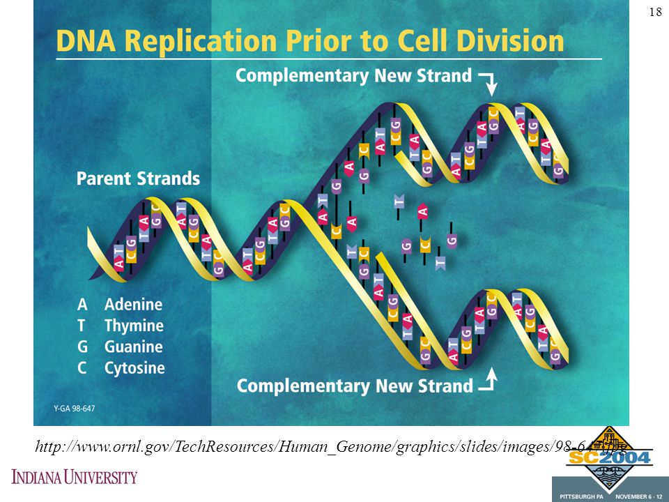
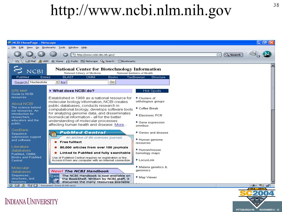
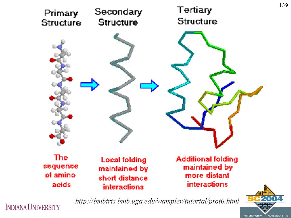
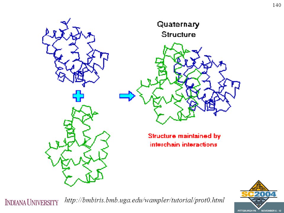
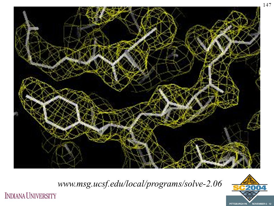
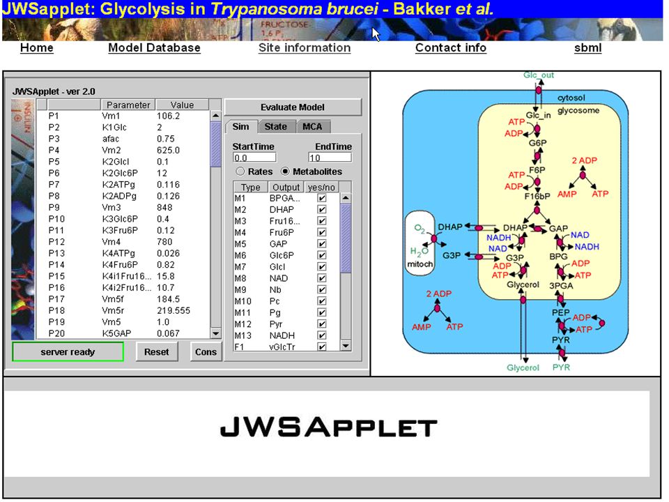
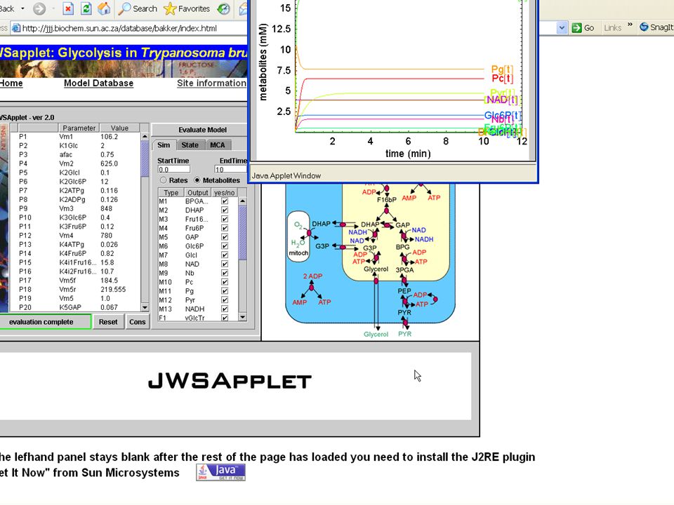


![. Protein Structure Prediction [Based on Structural Bioinformatics, section VII]](/16/5116302/big_thumb.jpg ". Protein Structure Prediction [Based on Structural Bioinformatics, section VII]>")


 The Mechanics of Alignments.>")