Download presentation
Presentation is loading. Please wait.

1
Chapter 5 Estimating Parameters From Observational Data Instructor: Prof. Wilson Tang CIVL 181 Modelling Systems with Uncertainties

2
Estimating Parameters From Observation Data REAL WORLD “POPULATION” (True Characteristics Unknown) Sample {x 1, x 2, …, x n } Sampling (Experimental Observations) Real Line -∞ < x < ∞ With Distribution f X (x) Random Variable X Inference On f X (x) f X (x) Statistical Estimation Role of sampling in statistical inference
 Sample {x 1, x 2, …, x n } Sampling (Experimental Observations) Real Line -∞ < x < ∞ With Distribution f X (x) Random Variable X Inference On f X (x) f X (x) Statistical Estimation Role of sampling in statistical inference")
3
Point Estimations of Parameters, e.g. , 2,, etc. a)Method of moments: equate statistical moments (e.g. mean, variance, skewness etc.) of the model to those of the sample. From Table 5.1 in pp 224 – 225 See e.g. 5.2 in p. 227
Method of moments: equate statistical moments (e.g. mean, variance, skewness etc.) of the model to those of the sample. From Table 5.1 in pp 224 – 225 See e.g. 5.2 in p")
4
Common Distributions and their Parameters

5
Common Distributions and their Parameters (Cont’d)
")
6
b) Method of maximum likelihood: Parameter = r.v. X with f x (x) Definition: L( ) = f X (x 1, ) f X (x 2, ) f X (x n, ), where x 1, x 2, x n are observed data Physical interpolation – the value of such that the likelihood function is maximized (i.e. likelihood of getting these data is maximized ) For practical purpose, the difference between the estimates obtained from these different methods would be small if sample size is sufficiently large.
 Definition: L( ) = f X (x 1, ) f X (x 2, ) f X (x n, ), where x 1, x 2, x n are observed data Physical interpolation – the value of such that the likelihood function is maximized (i.e. likelihood of getting these data is maximized ) For practical purpose, the difference between the estimates obtained from these different methods would be small if sample size is sufficiently large..")
7
b)Method of maximum likelihood (Cont ’ d): = 1 = 2 e - x x f X (x) X1X1 X2X2 GivenX 1 = 2 more likely Similarly,X 2 = 1 more likely Likelihood of depends on f X (x i ) and the x i ’s
Method of maximum likelihood (Cont ’ d): = 1 = 2 e - x x f X (x) X1X1 X2X2 GivenX 1 = 2 more likely Similarly,X 2 = 1 more likely Likelihood of depends on f X (x i ) and the x i ’s")
8
X: , What would you expect the value of X to be? As n Var(X) Before collections of data, X 1 is a r.v. = X X is r.v.
 Before collections of data, X 1 is a r.v. = X X is r.v..")
9
What is the distribution of X? n1n1 n2n2 n n 1 > n 2

10
Confidence interval of We would like to establish P(? < < ?) = 0.95 0.95 k 0.025 = 1.96 -1.96 0.025
 = k =")
11
Confidence interval of (Cont’d) Not a r.v. confidence interval /2 1 – k /2
 Not a r.v. confidence interval /2 1 – k /2")
12
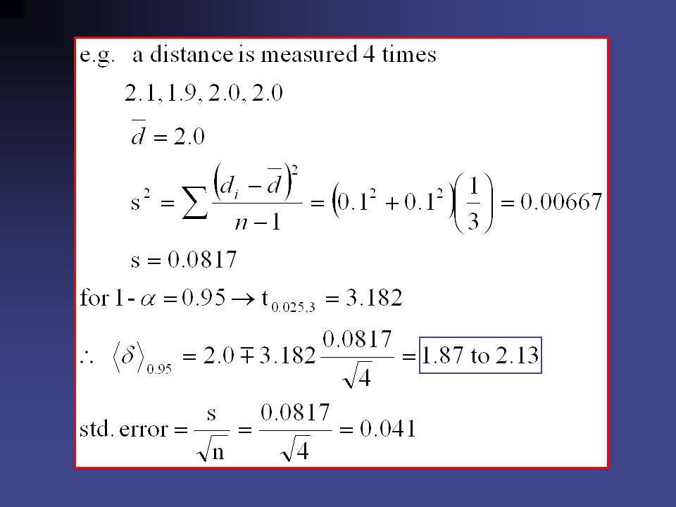
E5.5 Daily dissolved oxygen (DO) n = 30 observations s = 2.05 mg/l assume = x = 2.52 mg/l Determine 99% confidence interval of As confidence level interval <> n <>
 n = 30 observations s = 2.05 mg/l assume = x = 2.52 mg/l Determine 99% confidence interval of As confidence level interval <> n <> ")
13
Confidence Interval of when is unknown Small f Large f N(0,1) 0 known
 0 known")
14
/2 p t /2,f 0 (for known case)
")
15
E5.9 Traffic survey on speed of vehicles. Suppose we would like to determine the mean vehicle velocity to within 2 kph with 99 % confidence. How many vehicles should be observed? Assume = 3.58 from previous study Scatter 2.58 What if not known, but sample std. dev. expected to s = 3.58 and desired to be with 2 ?

16
E5.9 (Cont’d) Compare with n 21 for known
 Compare with n 21 for known")
17
Lower confidence limit Upper confidence limit 1 – kk Not /2 known unknown

18
- Similar to estimations of

20
What about an area? B C D

22
In general, r1r1 r2r2 h

23
Interval Estimation of 2 sample variance 2 statistics – confidence level n – no. of sample

24
E 5.13 DO data: n = 30, s 2 = 4.2

25
Estimation of proportions

26
10 out of 50 specimens do not have pass CBR requirement. E 5.14

27
Review on Chapter 5

Similar presentations


 from which the sample is drawn.>")


=“geometric distribution”), 9-R9(a,b) Recommended Questions: 9.1, 9.8, 9.20, 9.23, 9.25.>")


>")


