1. 4/3

2. (FO)MDPs: The plan General model has no initial state; complex cost and reward functions, and finite/infinite/indefinite horizons Standard algorithms are Value and Policy iteration –Have to look at the entire state space Can be made even more general with –Partial observability (POMDPs) –Continuous state spaces –Multiple agents (DECPOMDPS/MDPS) –Durative actions Conurrent MDPs Semi-MDPs Directions –Efficient algorithms for special cases TODAY & 4/10 –Combining “Learning” of the model and “planning” with the model Reinforcement Learning—4/8

3. Markov Decision Process (MDP)  S : A set of states  A : A set of actions  P r(s’|s,a): transition model (aka M a s,s’ )  C (s,a,s’): cost model  G : set of goals  s 0 : start state   : discount factor  R ( s,a,s’): reward model Value function: expected long term reward from the state Q values: Expected long term reward of doing a in s V(s) = max Q(s,a) Greedy Policy w.r.t. a value function Value of a policy Optimal value function

4. Examples of MDPs  Goal-directed, Indefinite Horizon, Cost Minimization MDP Most often studied in planning community  Infinite Horizon, Discounted Reward Maximization MDP Most often studied in reinforcement learning  Goal-directed, Finite Horizon, Prob. Maximization MDP Also studied in planning community  Oversubscription Planning: Non absorbing goals, Reward Max. MDP Relatively recent model

5. SSPP—Stochastic Shortest Path Problem An MDP with Init and Goal states MDPs don’t have a notion of an “initial” and “goal” state. (Process orientation instead of “task” orientation) –Goals are sort of modeled by reward functions Allows pretty expressive goals (in theory) –Normal MDP algorithms don’t use initial state information (since policy is supposed to cover the entire search space anyway). Could consider “envelope extension” methods –Compute a “deterministic” plan (which gives the policy for some of the states; Extend the policy to other states that are likely to happen during execution –RTDP methods SSSP are a special case of MDPs where –(a) initial state is given –(b) there are absorbing goal states –(c) Actions have costs. All states have zero rewards A proper policy for SSSP is a policy which is guaranteed to ultimately put the agent in one of the absorbing states For SSSP, it would be worth finding a partial policy that only covers the “relevant” states (states that are reachable from init and goal states on any optimal policy) –Value/Policy Iteration don’t consider the notion of relevance –Consider “heuristic state search” algorithms Heuristic can be seen as the “estimate” of the value of a state.

6.   Define J*(s) {optimal cost} as the minimum expected cost to reach a goal from this state.  J* should satisfy the following equation: Bellman Equations for Cost Minimization MDP (absorbing goals)[also called Stochastic Shortest Path] Q*(s,a)

7.   Define V*(s) {optimal value} as the maximum expected discounted reward from this state.  V* should satisfy the following equation: Bellman Equations for infinite horizon discounted reward maximization MDP

8.   Define P*(s,t) {optimal prob.} as the maximum probability of reaching a goal from this state at t th timestep.  P* should satisfy the following equation: Bellman Equations for probability maximization MDP

9. Modeling Softgoal problems as deterministic MDPs Consider the net-benefit problem, where actions have costs, and goals have utilities, and we want a plan with the highest net benefit How do we model this as MDP? –(wrong idea): Make every state in which any subset of goals hold into a sink state with reward equal to the cumulative sum of utilities of the goals. Problem—what if achieving g1 g2 will necessarily lead you through a state where g1 is already true? –(correct version): Make a new fluent called “done” dummy action called Done-Deal. It is applicable in any state and asserts the fluent “done”. All “done” states are sink states. Their reward is equal to sum of rewards of the individual states.

10. Ideas for Efficient Algorithms.. Use heuristic search (and reachability information) –LAO*, RTDP Use execution and/or Simulation –“Actual Execution” Reinforcement learning (Main motivation for RL is to “learn” the model) –“Simulation” –simulate the given model to sample possible futures Policy rollout, hindsight optimization etc. Use “factored” representations –Factored representations for Actions, Reward Functions, Values and Policies –Directly manipulating factored representations during the Bellman update

11. Heuristic Search vs. Dynamic Programming (Value/Policy Iteration) VI and PI approaches use Dynamic Programming Update Set the value of a state in terms of the maximum expected value achievable by doing actions from that state. They do the update for every state in the state space –Wasteful if we know the initial state(s) that the agent is starting from Heuristic search (e.g. A*/AO*) explores only the part of the state space that is actually reachable from the initial state Even within the reachable space, heuristic search can avoid visiting many of the states. –Depending on the quality of the heuristic used.. But what is the heuristic? –An admissible heuristic is a lowerbound on the cost to reach goal from any given state –It is a lowerbound on V*!

12. Connection with Heuristic Search s0s0 G s0s0 G ?? s0s0 G ?? regular graph acyclic AND/OR graph cyclic AND/OR graph

13. Connection with Heuristic Search s0s0 G s0s0 G ?? s0s0 G ?? regular graph soln:(shortest) path A* acyclic AND/OR graph soln:(expected shortest) acyclic graph AO* [Nilsson’71] cyclic AND/OR graph soln:(expected shortest) cyclic graph LAO* [Hansen&Zil.’98] All algorithms able to make effective use of reachability information! Sanity check: Why can’t we handle the cycles by duplicate elimination as in A* search?

14. LAO* [Hansen&Zilberstein’98] 1.add s 0 in the fringe and in greedy graph 2.repeat  expand a state on the fringe (in greedy graph)  initialize all new states by their heuristic value  perform value iteration for all expanded states  recompute the greedy graph 3.until greedy graph is free of fringe states 4.output the greedy graph as the final policy

15. LAO* [Iteration 1] s0s0 G ?? s0s0 add s 0 in the fringe and in greedy graph

16. LAO* [Iteration 1] s0s0 G ?? s0s0 expand a state on fringe in greedy graph ??

17. LAO* [Iteration 1] s0s0 G ?? s0s0  initialise all new states by their heuristic values  perform VI on expanded states ?? h hhh J1J1

18. LAO* [Iteration 1] s0s0 G ?? s0s0 recompute the greedy graph ?? h hhh J1J1

19. LAO* [Iteration 2] s0s0 G ?? s0s0 expand a state on the fringe initialise new states ?? h hhh J1J1 h h

20. LAO* [Iteration 2] s0s0 G ?? s0s0 perform VI compute greedy policy ?? h hh J2J2 h h J2J2

21. LAO* [Iteration 3] s0s0 G ?? s0s0 expand fringe state ?? h h J2J2 h h J2J2 G

22. LAO* [Iteration 3] s0s0 G ?? s0s0 perform VI recompute greedy graph ?? h h J3J3 h h J3J3 G J3J3

23. LAO* [Iteration 4] s0s0 G ?? s0s0 ?? h J4J4 h h J4J4 G J4J4 h J4J4

24. s0s0 G ?? s0s0 ?? h J4J4 h h J4J4 G J4J4 h J4J4 Stops when all nodes in greedy graph have been expanded

25. Comments  Dynamic Programming + Heuristic Search  admissible heuristic ⇒ optimal policy  expands only part of the reachable state space  outputs a partial policy one that is closed w.r.t. to P r and s 0 Speedups expand all states in fringe at once perform policy iteration instead of value iteration perform partial value/policy iteration weighted heuristic: f = (1-w).g + w.h ADD based symbolic techniques (symbolic LAO*)

26. AO* search for solving SSP problems Main issues: -- Cost of a node is expected cost of its children -- The And tree can have LOOPS  Cost backup is complicated Intermediate nodes given admissible heuristic estimates --can be just the shortest paths (or their estimates)

27. LAO*--turning bottom-up labeling into a full DP

28. How to derive heuristics? Deterministic shortest route is a heuristic on the expected cost J*(s) But how do you compute it? –Idea 1: [Most likely outcome determinization] Consider the most likely transition for each action –Idea 2: [All outcome determinization] For each stochastic action, make multiple deterministic actions that correspond to the various outcomes –Which is admissible? Which is “more” informed? –How about Idea 3: [Sampling based determinization] Construct a sample determinization by “simulating” each stochastic action to pick the outcome. Find the cost of shortest path in that determinization Take multiple samples, and take the average of the shortest path. Determinization involves converting “And” arcs in the And/Or graph to “Or” arcs

29. Real Time Dynamic Programming [Barto, Bradtke, Singh’95]  Trial: simulate greedy policy starting from start state; perform Bellman backup on visited states  RTDP: repeat Trials until cost function converges Notice that you can also do the “Trial” above by executing rather than “simulating”. In that case, we will be doing reinforcement learning. (In fact, RTDP was originally developed for reinforcement learning)

30. RTDP Approach: Interleave Planning & Execution (Simulation) Start from the current state S. Expand the tree (either uniformly to k-levels, or non-uniformly—going deeper in some branches) Evaluate the leaf nodes; back-up the values to S. Update the stored value of S. Pick the action that leads to best value Do it {or simulate it}. Loop back. Leaf nodes evaluated by Using their “cached” values  If this node has been evaluated using RTDP analysis in the past, you use its remembered value else use the heuristic value  If not use heuristics to estimate a. Immediate reward values b. Reachability heuristics Sort of like depth-limited game-playing (expectimax) --Who is the game against? Can also do “reinforcement learning” this way  The M ij are not known correctly in RL

31. Min ? ? s0s0 JnJn JnJn JnJn JnJn JnJn JnJn JnJn Q n+1 (s 0,a) J n+1 (s 0 ) a greedy = a 2 Goal a1a1 a2a2 a3a3 RTDP Trial ?

32. Greedy “On-Policy” RTDP without execution  Using the current utility values, select the action with the highest expected utility (greedy action) at each state, until you reach a terminating state. Update the values along this path. Loop back—until the values stabilize

34. Comments  Properties if all states are visited infinitely often then J n → J*  Advantages Anytime: more probable states explored quickly  Disadvantages complete convergence is slow! no termination condition

35. Labeled RTDP [Bonet&Geffner’03]  Initialise J 0 with an admissible heuristic ⇒ J n monotonically increases  Label a state as solved if the J n for that state has converged  Backpropagate ‘solved’ labeling  Stop trials when they reach any solved state  Terminate when s 0 is solved sG high Q costs best action ) J(s) won’t change! sG ? t both s and t get solved together high Q costs

36. Properties  admissible J 0 ⇒ optimal J*  heuristic-guided explores a subset of reachable state space  anytime focusses attention on more probable states  fast convergence focusses attention on unconverged states  terminates in finite time

37. Recent Advances: Bounded RTDP [McMahan, Likhachev & Gordon’05]  Associate with each state Lower bound (lb): for simulation Upper bound (ub): for policy computation gap(s) = ub(s) – lb(s)  Terminate trial when gap(s) <   Bias sampling towards unconverged states proportional to P r(s’|s,a).gap(s’)  Perform backups in reverse order for current trajectory.

38. Recent Advances: Focused RTDP [Smith&Simmons’06] Similar to Bounded RTDP except a more sophisticated definition of priority that combines gap and prob. of reaching the state adaptively increasing the max-trial length Recent Advances: Learning DFS [Bonet&Geffner’06]  Iterative Deepening A* equivalent for MDPs  Find strongly connected components to check for a state being solved.

39. Other Advances  Ordering the Bellman backups to maximise information flow. [Wingate & Seppi’05] [Dai & Hansen’07]  Partition the state space and combine value iterations from different partitions. [Wingate & Seppi’05] [Dai & Goldsmith’07]  External memory version of value iteration [Edelkamp, Jabbar & Bonet’07]  …

40. Policy Gradient Approaches [Williams’92]  direct policy search parameterised policy Pr(a|s,w) no value function flexible memory requirements  policy gradient J(w)=E w [  t=0.. 1  t c t ] gradient descent (wrt w) reaches a local optimum continuous/discrete spaces parameterised policy Pr(a|s.w) …… parameters w state s action a Pr(a=a 1 |s,w) Pr(a=a 2 |s,w) Pr(a=a k |s,w) …. non-stationary

41. Policy Gradient Algorithm  J(w)=E w [  t=0.. 1  t c t ] (failure prob.,makespan, …)  minimise J by computing gradient stepping the parameters away w t+1 = w t −  r J(w)  until convergence  Gradient Estimate [Sutton et.al.’99, Baxter & Bartlett’01]  Monte Carlo estimate from trace s 1, a 1, c 1, …, s T, a T, c T e t+1 = e t + r w log Pr(a t+1 |s t,w t ) w t+1 = w t -  t c t e t+1

42. Policy Gradient Approaches  often used in reinforcement learning partial observability model free ( P r(s’|s,a), P r(o|s) are unknown) to learn a policy from observations and costs Reinforcement Learner …… Pr(a|o,w) Pr(a=a 1 |o,w) Pr(a=a 2 |o,w) Pr(a=a k |o,w) …. world/simulator P r(s’|s,a) P r(o|s) observation o cost c action a

43. Modeling Complex Problems  Modeling time continuous variable in the state space discretisation issues large state space  Modeling concurrency many actions may execute at once large action space  Modeling time and concurrency large state and action space!! J(s) t t

44. Ideas for Efficient Algorithms.. Use heuristic search (and reachability information) –LAO*, RTDP Use execution and/or Simulation –“Actual Execution” Reinforcement learning (Main motivation for RL is to “learn” the model) –“Simulation” –simulate the given model to sample possible futures Policy rollout, hindsight optimization etc. Use “factored” representations –Factored representations for Actions, Reward Functions, Values and Policies –Directly manipulating factored representations during the Bellman update

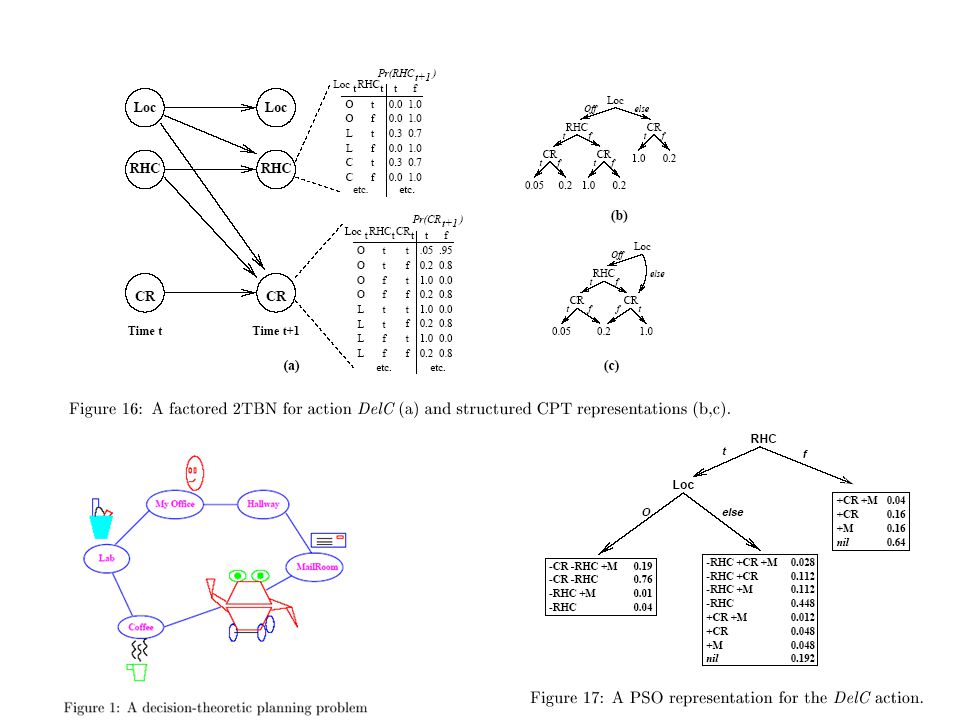
45. Factored Representations: Actions Actions can be represented directly in terms of their effects on the individual state variables (fluents). The CPTs of the BNs can be represented compactly too! –Write a Bayes Network relating the value of fluents at the state before and after the action Bayes networks representing fluents at different time points are called “Dynamic Bayes Networks” We look at 2TBN (2-time-slice dynamic bayes nets) Go further by using STRIPS assumption –Fluents not affected by the action are not represented explicitly in the model –Called Probabilistic STRIPS Operator (PSO) model

46. Action CLK

47. Envelope Extension Methods For each action, take the most likely outcome and discard the rest. Find a plan (deterministic path) from Init to Goal state. This is a (very partial) policy for just the states that fall on the maximum probability state sequence. Consider states that are most likely to be encountered while traveling this path. Find policy for those states too. Tricky part is to show that we can converge to the optimal policy

51. Factored Representations: Reward, Value and Policy Functions Reward functions can be represented in factored form too. Possible representations include –Decision trees (made up of fluents) –ADDs (Algebraic decision diagrams) Value functions are like reward functions (so they too can be represented similarly) Bellman update can then be done directly using factored representations..

53. SPUDDs use of ADDs

54. Direct manipulation of ADDs in SPUDD

58. Policy Rollout: Time Complexity …… Following PR[π,h,w] s s … … … … … Trajectories under  a1 an To compute PR[π,h,w](s) for each action we need to compute w trajectories of length h Total of |A|hw calls to the simulator

59. Policy Rollout  Often π’ is significantly better than π. I.e. one step of policy iteration can provide substantial improvement  Using simulation to approximate π’ is known as policy rollout PolicyRollout(s, π, h, w)  FOR each action a, Q’(a) = EstimateQ(s, a, π, h, w)  RETURN arg max a Q’(a)  We will denote the rollout policy by PR[π,h,w]  Note that PR[π,h,w] is stochastic  Questions:  What is the complexity of computing PR[π,h,w](s)?  Can we approximate k iterations of policy iteration using sampling?  How good is the rollout policy compared to the policy iteration improvement?

60. Multi-Stage Policy Rollout …… Following PR[PR[π,h,w],h,w] s s … … … … … Trajectories under PR[ π,h,w] a1 an Approximates policy resulting from two steps of PI. Requires (|A|hw) 2 calls to the simulator In general exponential in the number of PI iterations Each step requires |A|hw simulator calls

61. Policy Rollout: Quality  How good is PR[π,h,w](s) compared to π’?  In general for a fixed h and w there is always an MDP such that the quality of the rollout policy is arbitrarily worse than π’.  If we make an assumption about the MDP, then it is possible to select h and w so that the rollout quality is close to π’.  This is a bit involved.  In your homework you will solve a related problem.  Choose h and w so that with high probability PR[π,h,w](s) selects an action that maximizes Q π (s,a)

62. Rollout Summary  We often are able to write simple, mediocre policies  Network routing policy  Policy for card game of Hearts  Policy for game of Backgammon  Solitaire playing policy  Policy rollout is a general and easy way to improve upon such policies  Often observe substantial improvement, e.g.  Compiler instruction scheduling  Backgammon  Network routing  Combinatorial optimization  Game of GO  Solitaire

63. Example: Rollout for Go  Go is a popular board game for which there are still no highly-ranked computer programs  High branching factor  Difficult to design heuristics  Unlike Chess where the best computers compete with the best humans  What if we play Go using level-1 rollouts of the random policy?  With a few additional tweaks you get the best go program to date! (CrazyStone, winner of 11 th Computer Go Olympiad) http://remi.coulom.free.fr/CrazyStone/

64. FF-Replan: A Baseline for Probabilistic Planning Sungwook Yoon Alan fern Robert Givan FF-Replan : Sungwook Yoon

65. Replanning Approach Deterministic Planner for Probabilistic Planning? Winner of IPPC-2004 and (unofficial) winner of IPPC-2006 Why was it conceived? Why it worked? – Domain by domain analysis Any extension? FF-Replan : Sungwook Yoon

66. IPPC-2004 Pre-released Domains Blocksworld Boxworld FF-Replan : Sungwook Yoon

67. IPPC Performance Test -Client Server Interaction -The problem definition is known apriori -Performance is recorded in the server log -For one problem, 30 repetitive test is conducted FF-Replan : Sungwook Yoon

68. Single Outcome Replanning (FFR s ) Natural approach given the competition setting and the domains, Intro to AI (Russell and Norvig) – Hash state-action mapping Replace probabilistic effects with deterministic effect Ground Goal Action Effect 1 Effect 2 Effect 3 Probability 1 Probability 2 Probability 3 ActionEffect 2 C B A FF-Replan : Sungwook Yoon

69. IPPC-2004 Domains Blocksworld Boxworld Fileworld Tireworld Tower of Hanoi ZenoTravel Exploding Blocksworld FF-Replan : Sungwook Yoon

70. IPPC-2004 Results NMR C J1ClassyNMRmGPTCFFR S FFR A BW2522702553012030210270 Box1341501000300150 File---33031429 Zeno---30 0 Tire-r---30 Tire-g---9163077 TOH---1500011 Exploding ---00035 Human Control Knowledge 2 nd Place Winners Learned Knowledge NMR Non-Markovian Reward Decision Process Planner ClassyApproximate Policy Iteration with a Policy Language Bias mGPTHeuristic Search Probabilistic Planning CSymbolic Heuristic Search Numbers : Successful Runs

71. Reason of the Success Determinization and efficient pre-processing of complex planning language – Input language is quite complex (PPDDL) – Classic planning has developed efficient preprocessing techniques on complex input language and scales well – Grounding goal also helped Classic planning takes hard time dealing with lifted goals The domains in the competition – 17 of 20 problems were dead-end free – Amenable to Replanning approach FF-Replan : Sungwook Yoon

72. All Outcome Replanning (FFR A ) Selecting one outcome is troublesome – Which outcome to take? – Let’s use all the outcomes – All we have to do is translating a deterministic action to the original probabilistic action during the server-client interaction with MDPSIM – Novel approach Action Effect 1 Effect 2 Effect 3 Probability 1 Probability 2 Probability 3 Action1Effect 1 Action2Effect 2 Action3Effect 3 FF-Replan : Sungwook Yoon

73. IPPC-2006 Domains Blocksworld Exploding Blocksworld ZenoTravel Tireworld Elevator Drive PitchCatch Schedule Random Randomly generate syntactically correct domain – E.g., Don’t delete facts that are not in the precondition Randomly generate a state – This is initial state Take random walk from the state, using the random domain The resulting state is a goal state – There is at least a path from the initial state to the goal state If the probability of the path is bigger than α, then stop, otherwise take a random walk again Special reset action is provided that take any state to the initial state FF-Replan : Sungwook Yoon

74. IPPC-2006 Results FFR A FPGFOALPsfDPParagraphFFR S BW866310029077 Zenotravel100270777 Random1006500573 Elevator93761000093 Exploding52432431 52 Drive71560090 Schedule51540010 PitchCatch54230000 Tire82758209169 FPGFactored Policy Gradient Planner FOALPFirst Order Approximate Linear Programming sfDP Symbolic Stochastic Focused Dynamic Programming with Decision Diagrams ParagraphA Graphplan Based Probabilistic Planner Numbers : Percentage of Successful Runs

75. Discussion Novel all-outcome replanning technique outperforms naïve replanner The replanner performed well even on the “real” probabilistic domains – Drive – The complexity of the domain might have contributed to this phenomenon Replanner did not win the domains where it is supposed to be very best – Blocksworld FF-Replan : Sungwook Yoon

76. Weakness of the Replanning Ignorance of the probabilistic effects – Try not to use actions with detrimental effects – Detrimental effects can sometimes easily be found Ignorance of prior planning during replanning – Plan Stability Work by Fox, Gerevini, Long and Serina No learning – There is an obvious learning opportunity, since it solves a problem repetitively FF-Replan : Sungwook Yoon

77. Potential improvements Intelligent Replanning Policy rollout Policy learning Hindsight Optimization During (determinized) planning, when it meets the previous seen state, stop planning – May reduce the replanning time State FF Replan Average Select Max A1A2 Reward FF Replan Average Reward Hashing state-action mapping can be viewed as partial policy Currently, the mapping is always fixed When there is a failure, we can update the policy, that is, give penalty to the state-actions in the failure trajectory During planning, try not to use those actions in those states – E.g., after explosion in the exploding-blocksworld, do not use putdown action state action Action outcome that really will happen Goal State FF-Replan : Sungwook Yoon