1. FP-growth

2. Challenges of Frequent Pattern Mining Improving Apriori Fp-growth Fp-tree Mining frequent patterns with FP-tree Visualization of Association Rules

3. Challenges of Frequent Pattern Mining Challenges Multiple scans of transaction database Huge number of candidates Tedious workload of support counting for candidates Improving Apriori: general ideas Reduce passes of transaction database scans Shrink number of candidates Facilitate support counting of candidates

4. Transactional Database

6. Association Rule Mining Find all frequent itemsets Generate strong association rules from the frequent itemsets Apriori algorithm is mining frequent itemsets for Boolean associations rules

7. Improving Apriori Reduce passes of transaction database scans Shrink number of candidates Facilitate support counting of candidates Use constraints

8. The Apriori Algorithm — Example Database D Scan D C1C1 L1L1 L2L2 C2C2 C2C2 C3C3 L3L3

9. Apriori + Constraint Database D Scan D C1C1 L1L1 L2L2 C2C2 C2C2 C3C3 L3L3 Constraint: Sum{S.price} < 5

10. Push an Anti-monotone Constraint Deep Database D Scan D C1C1 L1L1 L2L2 C2C2 C2C2 C3C3 L3L3 Constraint: Sum{S.price} < 5

11. Hash-based technique The basic idea in hash coding is to determine the address of the stored item as some simple arithmetic function content Map onto a subspace of allocated addresses using a hash function Assume the allocated address range from b to n+b-1, the hashing function may take h=(a mod n)+b In order to create a good pseudorandom number, n ought to be prime

12. Two different keywords may have equal hash addresses Partition the memory into buckets, and to address each bucket One address is mapped into one bucket

13. When scanning each transition in the database to generate frequent 1-itemsets, we can generate all the 2-itemsets for each transition and hash them into different buckets of the hash table We use h=a mod n, a address, n < the size of C 2

14. A 2-itemset whose bucket count in the hash table is below the support threshold cannot be frequent, and should be removed from the candidate set

15. Transaction reduction A transaction which does not contain frequent k-itemsets should be removed from the database for further scans

16. Partitioning First scan: Subdivide the transactions of database D into n non overlapping partitions If the minimum support in D is min_sup, then the minimum support for a partition is min_sup * number of transactions in that partition Local frequent items are determined A local frequent item my not by a frequent item in D Second scan: Frequent items are determined from the local frequent items

17. Partitioning First scan: Subdivide the transactions of database D into n non overlapping partitions If the minimum support in D is min_sup, then the minimum support for a partition is min_sup * number of transactions in D / number of transactions in that partition Local frequent items are determined A local frequent item my not by a frequent item in D Second scan: Frequent items are determined from the local frequent items

18. Sampling Pick a random sample S of D Search for local frequent items in S Use a lower support threshold Determine frequent items from the local frequent items Frequent items of D may be missed For completeness a second scan is done

19. Is Apriori fast enough? Basics of Apriori algorithm Use frequent (k-1)-itemsets to generate k- itemsets candidates Scan the databases to determine frequent k- itemsets

20. It is costly to handle a huge number of candidate sets If there are 10 4 frequent 1-itemsts, the Apriori algorithm will need to generate more than 10 7 2-itemsets and test their frequencies

21. To discover a 100-itemset 2 100 -1 candidates have to be generated 2 100 -1=1.27*10 30 (Do you know how big this number is?).... 7* � 10 27  number of atoms of a person 6 � *10 49  number of atoms of the earth 10 78  number of the atom of the universe

22. Bottleneck of Apriori Mining long patterns needs many passes of scanning and generates lots of candidates Bottleneck: candidate-generation-and-test Can we avoid candidate generation? May some new data structure help?

23. Mining Frequent Patterns Without Candidate Generation Grow long patterns from short ones using local frequent items “abc” is a frequent pattern Get all transactions having “abc”: DB|abc “d” is a local frequent item in DB|abc  abcd is a frequent pattern

24. Construct FP-tree from a Transaction Database {} f:4c:1 b:1 p:1 b:1c:3 a:3 b:1m:2 p:2m:1 Header Table Item frequency head f4 c4 a3 b3 m3 p3 min_support = 3 TIDItems bought (ordered) frequent items 100{f, a, c, d, g, i, m, p}{f, c, a, m, p} 200{a, b, c, f, l, m, o}{f, c, a, b, m} 300 {b, f, h, j, o, w}{f, b} 400 {b, c, k, s, p}{c, b, p} 500 {a, f, c, e, l, p, m, n}{f, c, a, m, p} 1.Scan DB once, find frequent 1-itemset (single item pattern) 2.Sort frequent items in frequency descending order, f-list 3.Scan DB again, construct FP-tree F-list=f-c-a-b-m-p

25. Benefits of the FP-tree Structure Completeness Preserve complete information for frequent pattern mining Never break a long pattern of any transaction Compactness Reduce irrelevant info—infrequent items are gone Items in frequency descending order: the more frequently occurring, the more likely to be shared Never be larger than the original database (not count node-links and the count field) There exists examples of databases, where compression ratio could be over 100

26. The size of the FP-trees bounded by the overall occurrences of the frequent items in the database The height of the tree is bound by the maximal number of frequent items in a transaction

27. Partition Patterns and Databases Frequent patterns can be partitioned into subsets according to f-list f-list=f-c-a-b-m-p Patterns containing p Patterns having m but no p … Patterns having c but no a nor b, m, p Pattern f Completeness and non-redundency

28. Find Patterns Having p From p-conditional Database Starting at the frequent item header table in the FP-tree Traverse the FP-tree by following the link of each frequent item p Accumulate all of transformed prefix paths of item p to form p’s conditional pattern base Conditional pattern bases itemcond. pattern base cf:3 afc:3 bfca:1, f:1, c:1 mfca:2, fcab:1 pfcam:2, cb:1 {} f:4c:1 b:1 p:1 b:1c:3 a:3 b:1m:2 p:2m:1 Header Table Item frequency head f4 c4 a3 b3 m3 p3

29. From Conditional Pattern-bases to Conditional FP-trees For each pattern-base Accumulate the count for each item in the base Construct the FP-tree for the frequent items of the pattern base m-conditional pattern base: fca:2, fcab:1 {} f:3 c:3 a:3 m-conditional FP-tree All frequent patterns relate to m m, fm, cm, am, fcm, fam, cam, fcam -> associations   {} f:4c:1 b:1 p:1 b:1c:3 a:3 b:1m:2 p:2m:1 Header Table Item frequency head f4 c4 a3 b3 m3 p3

30. Recursion: Mining Each Conditional FP-tree {} f:3 c:3 a:3 m-conditional FP-tree Cond. pattern base of “am”: (fc:3) {} f:3 c:3 am-conditional FP-tree Cond. pattern base of “cm”: (f:3) {} f:3 cm-conditional FP-tree Cond. pattern base of “cam”: (f:3) {} f:3 cam-conditional FP-tree

31. itemconditional pattern baseconditional FP-tree

32. Mining Frequent Patterns With FP-trees Idea: Frequent pattern growth Recursively grow frequent patterns by pattern and database partition Method For each frequent item, construct its conditional pattern-base, and then its conditional FP-tree Repeat the process on each newly created conditional FP-tree Until the resulting FP-tree is empty, or it contains only one path—single path will generate all the combinations of its sub-paths, each of which is a frequent pattern

34. Experiments: FP-Growth vs. Apriori Data set T25I20D10K

35. Advantage when support decrease No prove advantage is shown by experiments with artificial data

36. Advantages of FP-Growth Divide-and-conquer: decompose both the mining task and DB according to the frequent patterns obtained so far leads to focused search of smaller databases Other factors no candidate generation, no candidate test compressed database: FP-tree structure no repeated scan of entire database basic ops—counting local freq items and building sub FP-tree, no pattern search and matching

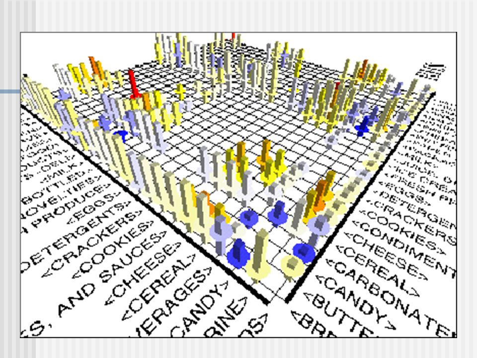
37. Visualization of Association Rules: Plane Graph

38. Visualization of Association Rules: Rule Graph

40. Challenges of Frequent Pattern Mining Improving Apriori Fp-growth Fp-tree Mining frequent patterns with FP-tree Visualization of Association Rules

41. Clustering k-means, EM