1. Class 2 Statistical Inference Lionel Nesta Observatoire Français des Conjonctures Economiques Lionel.nesta@ofce.sciences-po.fr CERAM February-March-April 2008

2. Hypothesis Testing

3. The Notion of Hypothesis in Statistics  Expectation  An hypothesis is a conjecture, an expected explanation of why a given phenomenon is occurring  Operational -ity  An hypothesis must be precise, univocal and quantifiable  Refutability  Le result of a given experiment must give rise to either the refutation or the corroboration of the tested hypothesis  Replicability  Exclude ad hoc, local arrangements from experiment, and seek universality

4. Examples of Good and Bad Hypotheses « The stakes Peugeot and Citroen have the same variance » « God exists! » « In general, the closure of a given production site in Europe is positively associated with the share price of a given company on financial markets. » « Knowledge has a positive impact on economic growth »    

5. Hypothesis Testing  In statistics, hypothesis testing aims at accepting or rejecting a hypothesis  The statistical hypothesis is called the “null hypothesis” H 0  The null hypothesis proposes something initially presumed true.  It is rejected only when it becomes evidently false, that is, when the researcher has a certain degree of confidence, usually 95% to 99%, that the data do not support the null hypothesis.  The alternative hypothesis (or research hypothesis) H 1 is the complement of H 0.

6. Hypothesis Testing  There are two kinds of hypothesis testing:  Homogeneity test compares the means of two samples.  H 0 : Mean( x ) = Mean( y ) ; Mean( x ) = 0  H 1 : Mean( x ) ≠ Mean( y ) ; Mean( x ) ≠ 0  Conformity test looks at whether the distribution of a given sample follows the properties of a distribution law (normal, Gaussian, Poisson, binomial).  H 0 : ℓ( x ) = ℓ*( x )  H 1 : ℓ( x ) ≠ ℓ*( x )

7. The Four Steps of Hypothesis Testing 1.Spelling out the null hypothesis H 0 et and the alternative hypothesis H 1. 2.Computation of a statistics corresponding to the distance between two sample means (homogeneity test) or between the sample and the distribution law (conformity test). 3.Computation of the (critical) probability to observe what one observes. 4.Conclusion of the test according to an agreed threshold around which one arbitrates between H 0 and H 1.

8. The Logic of Hypothesis Testing  We need to say something about the reliability (or representativeness) of a mean  Large number theory; Central limit theorem  The notion of confidence interval  Once done, we can whether two mean are alike  If so (not), their confidence intervals are (not) overlapping

9. Statistical Inference  In real life calculating parameters of populations is prohibitive because populations are very large.  Rather than investigating the whole population, we take a sample, calculate a statistic related to the parameter of interest, and make an inference.  The sampling distribution of the statistic is the tool that tells us how close is the statistic to the parameter.

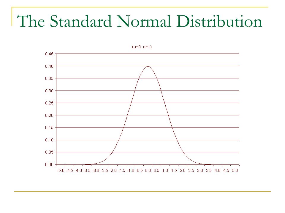
10. Prerequisite Standard Normal Distribution

11. Two Prerequisites  Large number theory  Large number theory tells us that the sample mean will converge to the population (true) mean as the sample size increases.  Central Limit Theorem  Central Limit Theorem tells us that for many samples of like and sufficiently large size, the histogram of these sample means will appear to be a normal distribution.

12. The Dice Experiment ValueP( X = x ) 11/6 2 3 4 5 6

13. The Dice Experiment (n = 2)

14. 1 1.5 2.0 2.5 3.0 3.5 4.0 4.5 5.0 5.5 6.0 6/36 5/36 4/36 3/36 2/36 1/36

15. The Normal Distribution In probability, a random variable follows a normal distribution law (also called Gaussian, Laplace-Gauss distribution law) of expectation μ and standard deviation σ if its probability density function (pdf) is such that This law is written N (μ,σ ²). The density function of a normal distribution is symmetrical.

16. Normal Distributions For Different values of μ and σ

17. The standard normal distribution, also called Z distribution, represents a probability density function with mean μ = 0 and standard deviation σ = 1. It is written as N (0,1). All random variable following a normal law can be standardized via the following transformation The Standard Normal Distribution

19. 68% of observations 95% of observations 99.7% of observations

20. The Standard Normal Distribution 95% of observations 2.5%

21. P(Z ≥ 0) P(Z < 0) The Standard Normal Distribution (z scores)

22. P(Z ≥ 0.51) Probability of an event (z = 0.51)

23.  The z-score is used to compute the probability of obtaining an observed score.  Example  Let z = 0.51. What is the probability of observing z=0.51?  It is the probability of observing z ≥ 0.51: P(z ≥ 0.51) = ??

24. Standard Normal Distribution Table z0.000.010.020.030.040.050.060.070.080.09 0.00.5000.4960.4920.4880.4840.4800.4760.4720.4680.464 0.10.4600.4560.4520.4480.4440.4400.4360.4330.4290.425 0.20.4210.4170.4130.4090.4050.4010.3970.3940.3900.386 0.30.3820.3780.3750.3710.3670.3630.3590.3560.3520.348 0.40.3450.3410.3370.3340.3300.3260.3230.3190.3160.312 0.50.3090.3050.3020.2980.2950.2910.2880.2840.2810.278 0.60.2740.2710.2680.2640.2610.2580.2550.2510.2480.245 0.70.2420.2390.2360.2330.2300.2270.2240.2210.2180.215 0.80.2120.2090.2060.2030.2010.1980.1950.1920.1890.187 0.90.1840.1810.1790.1760.1740.1710.1690.1660.1640.161 1.00.1590.1560.1540.1520.1490.1470.1450.1420.1400.138 1.60.0550.0540.0530.0520.050 0.0490.0480.0470.046 1.90.0290.0280.027 0.026 0.0250.024 0.023 2.00.0230.022 0.021 0.020 0.019 0.018 2.50.006 0.005 2.90.002 0.001

25. Probability of an event (Z = 0.51)  The Z-score is used to compute the probability of obtaining an observed score.  Example  Let z = 0.51. What is the probability of observing z=0.51?  It is the probability of observing z ≥ 0.51: P(z ≥ 0.51)  P(z ≥ 0.51) = 0.3050

26. Example  Suppose that for a population students of a famous business school in Sophia-Antipolis, grades are distributed normal with an average of 10 and a standard deviation of 3. What proportion of them  Exceeds 12 ; Exceeds 15  Does not exceed 8 ; Does not exceed 12  Let the mean μ = 10 and standard deviation σ = 3:

27. Confidence Interval

28. Inverting the way of thinking  Until now, we have thought in terms of observations x and sample values μ and σ to produce the z score.  Let us now imagine that we do not know x, we know μ and σ. If we consider any interval, we can write: ??

29. Inverting the way of thinking  If z ∈[-2.55;+2.55] we know that 99% of z-scores will fall within the range  If z ∈[-1.64;+1.64] we know that 90% of z-scores will fall within the range  Let us now consider an interval which comprises 95% of observations. Looking at the z table, we know that z=1.96

30. Confidence Interval  In statistics, a confidence interval is an interval within which the value of a parameter is likely to be (the mean). Instead of estimating the parameter by a single value, an interval of likely estimates is given.  Confidence intervals are used to indicate the reliability of an estimate.  A1. The sample mean is a random variable following a normal distribution  A2.The sample values μ and σ are good approximation of the population values.

31.  If a random sample is drawn from any population,  the sampling distribution of the sample mean is approximately normal for a sufficiently large sample size.  The larger the sample size, the more closely the sampling distribution of will resemble a normal distribution. The Central Limit Theorem

32. Moments of Sample Mean: The Mean On average, the sample mean will be on target, that is, equal to the population mean.

33. Moments of Sample Mean: The Variance The standard deviation of the sample means represents the estimation error of the sample mean, and therefore it is called the standard error.

34. The Sampling Distribution of the Sample Mean

35. General definition Definition for 95% CI Definition for 90% CI Confidence Interval

36. Standard Normal Distribution and CI 90% of observations 95% of observations 99.7% of observations

37.  Let us draw a sample of 25 students from CERAM (n = 25), with X = 10 and σ = 3. Let us build the 95% CI Application of Confidence Interval

38. CERAM Average grades 95% of chances that the mean is indeed located within this interval 8.8 11.2

39.  Let us draw a sample of 25 students from CERAM (n = 25), with X = 10 and σ = 3. Let us build the 95% CI Application of Confidence Interval  Let us draw a sample of 25 students from HEC (n = 30), with X = 11.5 and σ = 4.7. Let us build the 95% CI

40. HEC Average grades 95% of chances that the mean is indeed located within this interval 9.8 13.2

41. Hypothesis Testing  Hypothesis 1 : Students from CERAM have an average grade which is not significantly different from 11  H 0 : μ( CERAM ) = 11  H 1 : μ( CERAM ) ≠ 11  Hypothesis 2 : Students from CERAM have similar grades as students from HEC  H 0 : μ( CERAM ) = μ( HEC )  H 1 : μ( CERAM ) ≠ μ( HEC ) I Accept H 0 and reject H 1

42. Comparing the Means Using CI’s HEC CERAM The Overlap of the two CIs means that at 95% level, the two means do not differ significantly.

43.  Thus far, we have assumed that we know both the mean and the standard deviation of the population. But in fact, we do not know them: both μ and σ are unknown.  The Student t statistics is then preferred to the z statistics. Its distribution is similar (identical to z as n → +∞). The CI becomes The Student Test

44.  Let us draw a sample of 25 students from CERAM (n = 25), with μ = 10 and σ = 3. Let us build the 95% CI Application of Student t to CI’s  Let us draw a sample of 25 students from HEC (n = 30), with μ = 11.5 and σ = 4.7. Let us build the 95% CI

45.  Import CERAM_LMC into SPSS  Produce descriptive statistics for sales; labour, and R&D expenses  Analyse  Statistiques descriptives  Descriptive  Options: choose the statistics you may wish  A newspaper writes that by and large, LMCs have 95,000 employees.  Test statistically whether this is true at 1% level  Test statistically whether this is true at 5% level  Test statistically whether this is true at 10% and 20% level  Write out H 0 and H 1  Analyse  Comparer les moyennes  Test t pour é chantillon unique  Options: 99; 95, 90% SPSS Application: Student t

46. SPSS Application: t test at 99% level

47. SPSS Application: t test at 95% level

48. SPSS Application: t test at 80% level

49. SPSS Results (at 1% level)

50. Critical probability  The confidence interval is designed in such a way that for each t statistics chosen, we define a share of observations which this CI is comprising.  For large n, when t = 1.96, we have 95% CI  For large n, when t = 2.55, we have 99% CI  Actually, for each t, there corresponds a share of observations  One can compute directly the t value from our observations as follows:

51. Critical probability  The confidence interval is designed in such a way that for each t statistics chosen, we define a share of observations which this CI is comprising.  For large n, when t = 1.96, we have 95% CI  For large n, when t = 2.55, we have 99% CI  Actually, for each t, there corresponds a share of observation  http://www.socr.ucla.edu/Applets.dir/T-table.html http://www.socr.ucla.edu/Applets.dir/T-table.html  One can compute directly the t value from our observations as follows:

52. Critical probability  With t = 1.552, I can conclude the following:  12% probability that μ belongs to the distribution where the population mean = 95,000  I have 12% chances to wrongly reject H 0  88% probability that μ belongs to another distribution where the population mean ≠ 95,000  I have 88% chances to rightly reject H 0 Shall I the accept or reject H0?

53. 6.1% 88.0%

54. Critical probability  With t = 1.552, I can conclude the following:  12% probability that μ belongs to the distribution where the population mean = 95,000  I have 12% chances to wrongly reject H 0  88% probability that μ belongs to another distribution where the population mean ≠ 95,000  I have 88% chances to rightly reject H 0 I accept H 0 !!!

55. Critical probability  The practice is to reject H 0 only when the critical probability is lower than 0.1, or 10%  Some are even more cautious and prefer to reject H 0 at a critical probability level of 0.05, or 5%.  In any case, the philosophy of the statistician is to be conservative.

56. A Direct Comparison of Means Using Student t  Another way to compare two sample means is to calculate the CI of the mean difference. If 0 does not belong to CI, then the two sample have significantly different means. Standard error, also called pooled variance

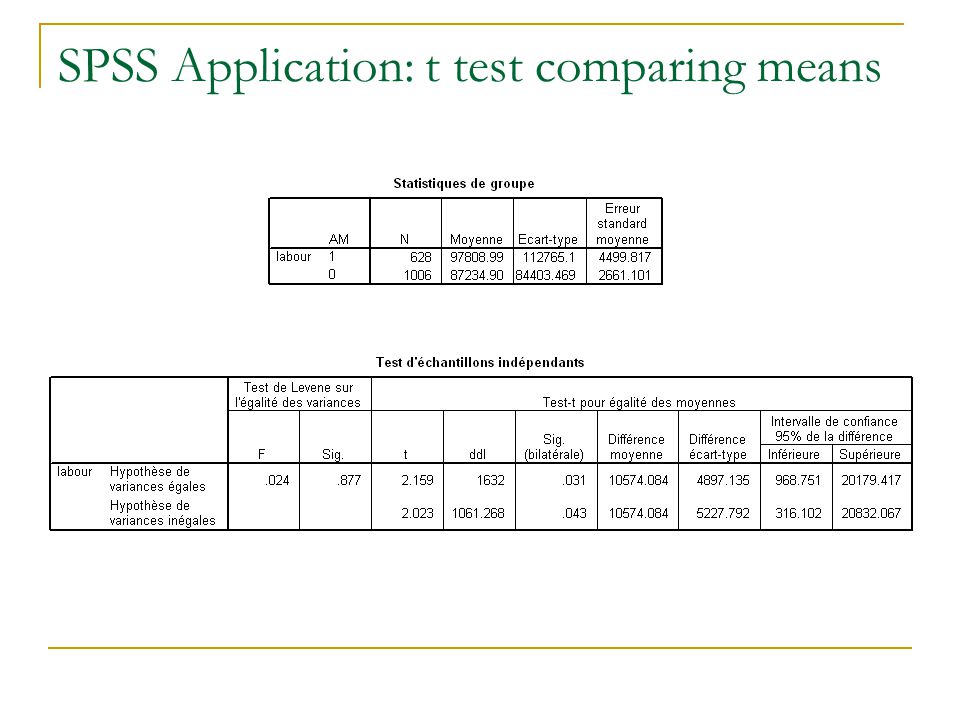
57.  Another newspaper argues that US companies are much larger than those from the rest of the world. Is this true?  Produce descriptive statistics labour comparing the two groups  Produce a group variables which equals 1 for US firms, 0 otherwise  This is called a dummy variable  Write out H 0 and H 1  Analyse  Comparer les moyennes  Test t pour é chantillon ind é pendants  What do you conclude at 5% level?  What do you conclude at 1% level? SPSS Application: t test comparing means