27 Inflation CHAPTER Notes and teaching tips: 4, 8, 17, 28, 36, 37, 52, 56, and 78. To view a full-screen figure during a class, click the red “expand”

27 Inflation CHAPTER Notes and teaching tips: 4, 8, 17, 28, 36, 37, 52, 56, and 78. To view a full-screen figure during a class, click the red “expand” button. To return to the previous slide, click the red “shrink” button. To advance to the next slide, click anywhere on the full screen figure.

Objectives After studying this chapter, you will able to
Distinguish between inflation and a change in the price level and between demand-pull inflation and cost-push inflation Explain the quantity theory of money Explain the short-run and long-run relationships between inflation and unemployment Explain the short-run and long-run relationships between inflation and interest rates

From Rome to Rio de Janeiro
Inflation is a very old problem and some countries even in recent times have experienced rates as high as 40 percent a month. Today, the Bank of Canada targets the inflation rate and keeps it low. But during the 1970s, the price level in Canada doubled. Why does inflation occur and do our expectations of inflation influence the economy? In targeting inflation, does the Bank of Canada face a tradeoff between inflation and unemployment? And how does inflation affect the interest rate?

Inflation: Demand-Pull and Cost-Push
Inflation is a process in which the price level is rising and money is losing value. Inflation is a rise in the price level, not in the price of a particular commodity. And inflation is an ongoing process, not a one-time jump in the price level. Stories and some data can make the impact of inflation real to students. Have them guess the price of something they buy (which has not changed much in its nature) when you were a student—possible items include a McDonald’s hamburger, a cup of coffee, an Economics Principles textbook, a pencil, a concert ticket, a gallon of gasoline, a semester’s tuition, and so on (prepare—make a list before you come in with actual prices you remember). Contrast the difference between a one-time price increase (such as tuition going up this year) with inflation (tuition going up every term). There is a good story that sometimes makes an impression: a very famous German economist in the 1950s used to keep in his pocket a British penny that he claimed he had received as change on a London bus, and would show it to students when lecturing on inflation. The point was that it was an 1840s Queen Victoria penny, and it illustrated the relative price stability in the UK as opposed to Germany (the story is true; any Brit who was a child in the 1950s will remember occasionally seeing Queen Victoria pennies). A possible contrast is with countries that have experienced rapid inflations, in many of which there are no coins in circulation at all (examples include Ghana, Indonesia, and Vietnam); ask students why rapid inflation countries often have no coins.

Figure 27.1 illustrates the distinction between inflation and a one-time rise in the price level.

The inflation rate is the percentage change in the price level. That is, where P1 is the current price level and P0 is last year’s price level, the inflation rate is [(P1 – P0)/P0]  100 Inflation can result from either an increase in aggregate demand or a decrease in aggregate supply and be Demand-pull inflation Cost-push inflation

Demand-Pull Inflation Demand-pull inflation is an inflation that results from an initial increase in aggregate demand. Demand-pull inflation may begin with any factor that increases aggregate demand. Two factors controlled by the government are increases in the quantity of money and increases in government purchases. A third possibility is an increase in exports. The potential difficulty with both demand-pull and cost-push inflation stories is how the one-time increase translates into an inflationary process. It is relatively easy to come up with stories as to why aggregate demand might shift continuously to the right, for example because of persistent and growing government budget deficits. What is a little harder is to provide a plausible story as to why the monetary authorities would continue to accommodate this with continuous increases in the quantity of money. Point out that this has been rare in Canada, and has tended to happen when the political situation was such that the Bank of Canada was not willing to be blamed for an increase in unemployment. In other countries, particularly where the central bank is less independent than in Canada, it has been more common.

Initial Effect of an Increase in Aggregate Demand Figure 27.2(a) illustrates the start of a demand-pull inflation. Starting from full employment, an increase in aggregate demand shifts the AD curve rightward.

The price level rises, real GDP increases, and an inflationary gap arises. The rising price level is the first step in the demand-pull inflation.

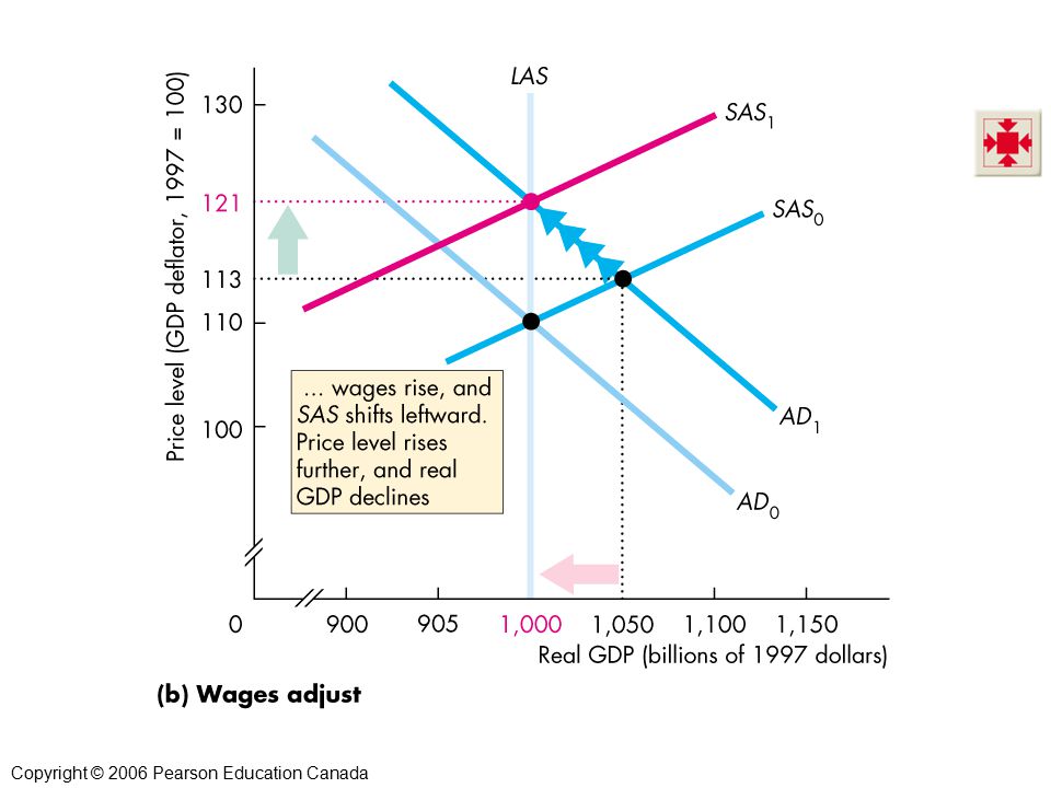
Money Wage Rate Response Figure 27.2(b) illustrates the money wage response. The money wages rises and the SAS curve shifts leftward. Real GDP decreases back to potential GDP but the price level rises further.

A Demand-Pull Inflation Process Figure 27.3 illustrates a demand-pull inflation spiral. Aggregate demand keeps increases and the process just described repeats indefinitely.

Although any of several factors can increase aggregate demand to start a demand-pull inflation, only an ongoing increase in the quantity of money can sustain it. Demand-pull inflation occurred in Canada during the late 1960s and early 1970s.

Cost-Push Inflation Cost-push inflation is an inflation that results from an initial increase in costs. There are two main sources of increased costs: 1. An increase in the money wage rate 2. An increase in the money price of raw materials, such as oil. The text gives a good description of the first oil price increase in the 1970s as a cost-push inflation, and contrasts it well with the Bank of Canada’s refusal to accommodate the second oil price increase in An explanation of how cost-push can be a more widespread cause of inflation in other countries can be given in terms of countries where labour is highly unionized, and in effect there are attempts by different interest groups to obtain shares of GDP that add up to more than 100 percent, with accommodation by a weak monetary authority. Such a process of repeated wage increases, inflation, and monetary accommodation can give rise to continuing inflation. Analysts often “explain” the cause of inflation by focusing attention on the good or service whose price increased the most during the most recent time period. This is incorrect; inflation is cased by monetary growth. One way to point out the fallacy is to use a baseball analogy. Several years ago the average number of home runs hit during major league baseball games increased. Virtually every commentator asked whether the ball had been doctored to make it livelier. No one explained the additional home runs by saying “home runs are higher because Parkin and Bade are hitting more home runs than last year.” To explain inflation, economists are looking for an explanation similar to the “doctored ball” explanation of the additional home runs, not an explanation that focuses on the performance of specific players.

Initial Effect of a Decrease in Aggregate Supply Figure 27.4 illustrates the start of cost-push inflation. A rise in the price of oil decreases short-run aggregate supply and shifts the SAS curve leftward.

Real GDP decreases and the price level rises—a combination called stagflation. The rising price level is the start of the cost-push inflation.

Aggregate Demand Response The initial increase in costs creates a one-time rise in the price level, not inflation. To create inflation, aggregate demand must increase.

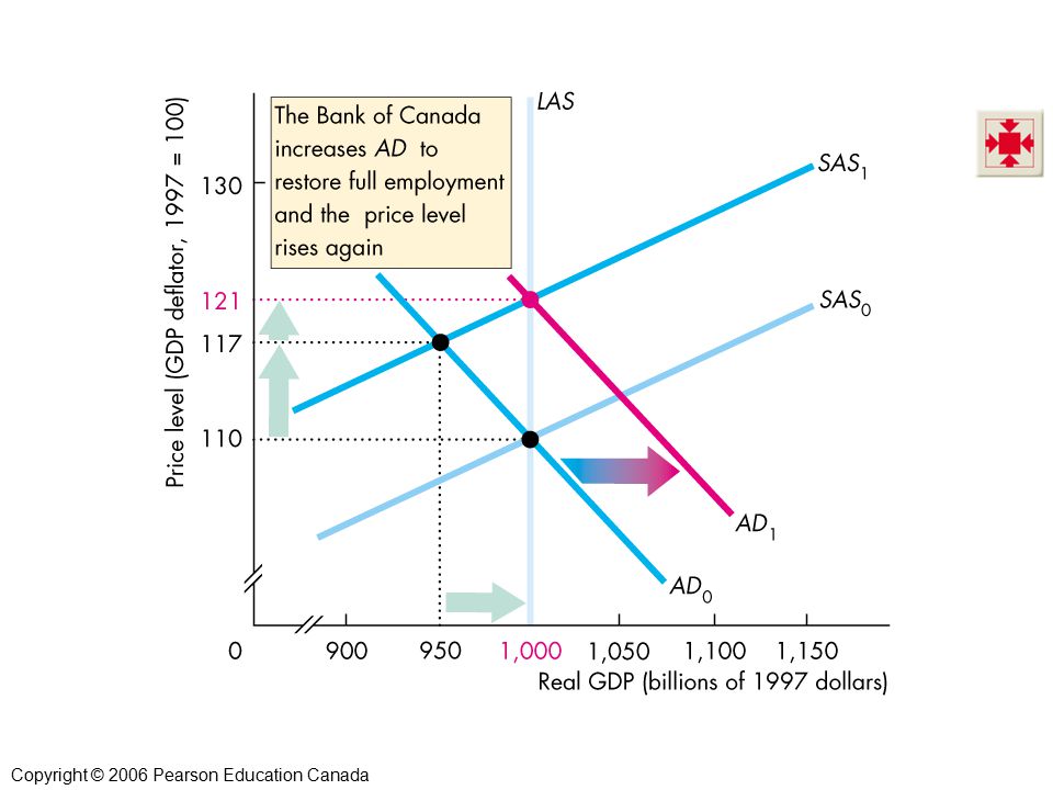
Figure 27.5 illustrates an aggregate demand response to stagflation, which might arise because the Bank of Canada stimulates demand to counter the higher unemployment rate and lower level of real GDP. Real GDP increases and the price level rises again.

A Cost-Push Inflation Process Figure 27.6 illustrates a cost-push inflation spiral.

If the oil producers raise the price of oil to try to keep its relative price higher, and the Bank of Canada responds with an increase in aggregate demand, a process of cost-push inflation continues. Cost-push inflation occurred in Canada during 1974–1978.

The Quantity Theory of Money
The quantity theory of money is the proposition that, in the long run, an increase in the quantity of money brings an equal percentage increase in the price level. The quantity theory of money is based on the velocity of circulation and the equation of exchange. The velocity of circulation is the average number of times in a year a dollar is used to purchase goods and services in GDP. Velocity of circulation. Emphasize that velocity is defined by the equation V = PY/M, and is not the average number of times a given piece of paper changes hands in a year. Nor is V the transactions velocity because most transactions are not payments for goods and services. (Transactions are twice PY because they also include payments for the services of factors of production, which equals PY, plus all the purely financial transactions such as buying and selling stocks, bonds, foreign currency, and real estates.) The quantity theory of money. Given that V is defined as PY/M, the equation of exchange, MV = PY is an identity. The quantity theory is not the equation of exchange but the propositions that (1) V is independent of M and (2) Y equals potential GDP, which is independent of M. Given these assumptions, the inflation rate equals the growth rate of the quantity of money. The quantity theory of hyperinflation. A possible exercise is to ask students whether we would expect the correlation between money growth and inflation to remain strong in a hyperinflation. Most will see that in a hyperinflation, velocity will increase. Emphasize that the level of velocity is greater in hyperinflation but if the inflation rate remains constant (and high) velocity also is constant (and high), so the quantity theory still holds. It does not hold in the move from low inflation to high inflation. The inflation rate overshoots the growth rate of the quantity of money.

Calling the velocity of circulation V, the price level P, real GDP Y, and the quantity of money M: V = PY ÷ M The equation of exchange states that MV = PY The equation of exchange becomes the quantity theory of money by making two assumptions: Velocity of circulation V is not influenced by M Potential GDP is not influenced by M

Given these two assumptions: P = (V/Y)M Because (V/Y) does not change when M changes, a change in M brings a proportionate change in P.

That is, the change in P, P, is related to the change in M, M, by the equation: P = (V/Y)M Divide this equation by P = (V/Y)M and the term (V/Y) cancels to give P/P = M/M P/P is the inflation rate and = M/M is the growth rate of the quantity of money.

Evidence on the Quantity Theory Canadian historical evidence is consistent with the quantity theory. On the average, the money growth rate exceeds the inflation rate. The money growth rate is correlated with the inflation rate. The next slide shows Figure 27.7, which summarizes the Canadian data on inflation and money growth for the years

International evidence shows a marked tendency for high money growth rates to be associated with high inflation rates. Figure 27.8(a) shows the evidence for 134 countries from 1990 to 2004. Figure 27.8(b) shows the evidence for 104 countries from 1990 to 2004.

Correlation, Causation, and Other Influences Correlation is not causation; money growth and inflation could be correlated because money growth causes inflation, or because inflation causes money growth, or because a third factor caused both. But the combination of historical, international, and other independent evidence gives us confidence that in the long run, money growth causes inflation. In the short run, the quantity theory is not correct; we need the AS-AD model to understand the links between money and inflation. The topic of this slide isn’t in the textbook. But you might argue that it ought to be. It is not hard to explain this material and we think it is important to do so.

Effects of Inflation Failure to anticipate inflation correctly results in unintended consequences that impose costs in both the labour market and the capital market. Unanticipated Inflation in the Labour Market Unanticipated inflation has two main consequences in the labour market: Redistribution of income Departure from full employment Numerical exercises can illustrate the income distribution effects very clearly. The wage example is very easy to do, simply in terms of an expected inflation rate, an agreed money wage, and then what the actual real wage will be if the actual inflation rate is different. The effects in the capital market are not quite as obvious, but are easily demonstrated with the impact of unanticipated inflation on house-buyers and mortgage lenders in the case of fixed-rate mortgages, which still remain dominant in Canada at least in part because inflation does tend to be low and fairly stable. It is important to make sure that students also get the notion that unanticipated inflation results in either over-full employment and more inflation, or less than full employment and cyclical unemployment. The idea of rational expectations is brought in here, and it is worth making sure that students have got clear what it means from the beginning. It is another case of unfortunate jargon; the issue is that the forecast based on rational expectations makes use of all information available, up to the point where expected improvements in accuracy are no more valuable than their cost. A rational expectation forecast is therefore not expected to be correct, it is the best that can be done at acceptable cost, and the errors in it are random. The important point for students to grasp is that there is nothing systematic, and therefore correctable, about the errors in a rational expectation forecast—implying that departures of reality from the forecast are truly unanticipated because they could not have been forecast. The costs of anticipated inflation are also worth some discussion. Students do not always fully appreciate that inflation means that the average level of prices is rising, but that individual prices may rise, fall, or stay the same. Try picking two items that have stable and unstable prices (e.g. a newspaper and a fast food meal during a price war), and then ask students how much time they would typically spend on a search before purchase if they were going to buy each; this will get across the shoe-leather cost idea. The tax and uncertainty effects are also amenable to numerical examples.

Effects of Inflation Redistribution of Income
Higher than anticipated inflation lowers the real wage rate and employers gain at the expense of workers. Lower than anticipated inflation raises the real wage rate and workers gain at the expense of employers.

Effects of Inflation Departure from Full Employment
Higher than anticipated inflation lowers the real wage rate, increases the quantity of labour demanded, makes jobs easier to find, and lowers the unemployment rate. Lower than anticipated inflation raises the real wage rate, decreases the quantity of labour demanded, and increases the unemployment rate.

Effects of Inflation Unanticipated Inflation in the Market for Financial Capital Unanticipated inflation has two main consequences in the market for financial capital: Redistribution of income Too much or too little lending and borrowing

Effects of Inflation Redistribution of Income
If the inflation rate is unexpectedly high, borrowers gain but lenders lose. If the inflation rate is unexpectedly low, lenders gain but borrowers lose.

Effects of Inflation Too Much or Too Little Lending and Borrowing
When the inflation rate is higher than anticipated, the real interest rate is lower than anticipated, and borrowers want to have borrowed more and lenders want to have loaned less. When the inflation rate is lower than anticipated, the real interest rate is higher than anticipated, and borrowers want to have borrowed less and lenders want to have loaned more.

Effects of Inflation Forecasting Inflation
To minimize the costs of incorrectly anticipating inflation, people form rational expectations about the inflation rate. A rational expectation is one based on all relevant information and is the most accurate forecast possible, although that does not mean it is always right; to the contrary, it will often be wrong.

Effects of Inflation Anticipated Inflation
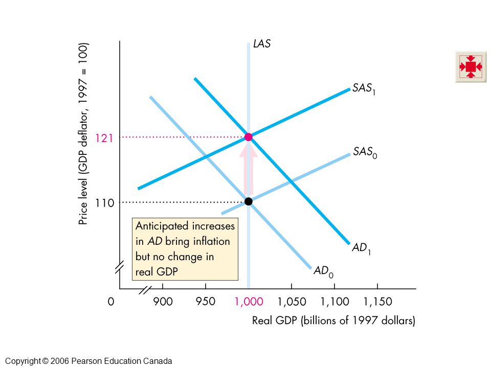
Figure 27.9 illustrates an anticipated inflation. Aggregate demand increases, but the increase is anticipated, so its effect on the price level is anticipated.

Effects of Inflation The money wage rate rises in line with the anticipated rise in the price level. The AD curve shifts rightward and the SAS curve shifts leftward so that the price level rises as anticipated and real GDP remains at potential GDP.

Effects of Inflation Unanticipated Inflation
If aggregate demand increases by more than expected, inflation is higher than expected. Money wages do not adjust enough, and the SAS curve does not shift leftward enough to keep the economy at full employment. Real GDP exceeds potential GDP. Wages eventually rise, which leads to a decrease in the short-run aggregate supply

Effects of Inflation The economy experiences more inflation as it returns to full employment. This inflation is like a demand-pull inflation.

Effects of Inflation If aggregate demand increases by less than expected, inflation is less than expected. Money wages rise too much and the SAS curve shifts leftward more than the AD curve shifts rightward. Real GDP is less than potential GDP. This inflation is like a cost-push inflation.

Effects of Inflation The Costs of Anticipated Inflation
Anticipated inflation occurs at full employment with real GDP equal to potential GDP. But anticipated inflation, particularly high anticipated inflation, inflicts three costs: Transactions costs Tax effects Increased uncertainty

Inflation and Unemployment: The Phillips Curve
A Phillips curve is a curve that shows the relationship between the inflation rate and the unemployment rate. There are two time frames for Phillips curves: The short-run Phillips curve The long-run Phillips curve The Phillips curve story nicely illustrates how progress is made in economics. The story starts in 1958 when Bill Phillips published his famous paper. At that time the mainstream economic model was the aggregate expenditure model presented in Chapter 25. The model was based on the assumption that the price level was constant, making the inflation rate zero. This assumption was not too unrealistic immediately after World War II. By 1955, though, the inflation rate began to creep higher and averaged 2.7 percent per year between 1956 and Inflation was beginning to be perceived as a problem, one that a model with a “fixed price level assumption” was poorly suited to solve. In this environment, economists gladly welcomed the simple, short-run Phillips curve, for it gave them a handle on inflation. They believed that they could predict the unemployment rate from their standard model and then combine this unemployment rate with the Phillips curve to determine the resulting inflation rate. The vital assumption in this procedure is that the Phillips curve captures a fixed tradeoff between the actual inflation rate and the unemployment rate that is part of the economy’s structure. This type of analysis reached its peak of popularity during the early and middle 1960s. But by 1967 it was under attack. On a theoretical level, Ned Phelps and Milton Friedman pointed out the flimsy justification behind the simple, fixed Phillips curve assumption. On an empirical level, the fixed Phillips curve failed as the inflation rate rose toward the end of the 1960s and into the 1970s: the unemployment rate did not fall as predicted by the fixed Phillips curve. At this point the idea of a long-run Phillips curve (as distinct from the short-run one) was developed. The concept that aggregate supply is an important component of macroeconomics was taking hold, as was the idea that short-run Phillips curves shift because of changes in people’s expectations. Thus the profession advanced significantly between the initial discussion of the Phillips curve and what students learn today. This advance was the result of the interaction between theory, suggesting that the idea of a fixed short-run Phillips curve was inadequate, and empirical work that reinforced the point that the simple, early approach was deficient.

The Short-Run Phillips Curve The short-run Phillips curve shows the tradeoff between the inflation rate and unemployment rate, holding constant 1. The expected inflation rate 2. The natural unemployment rate

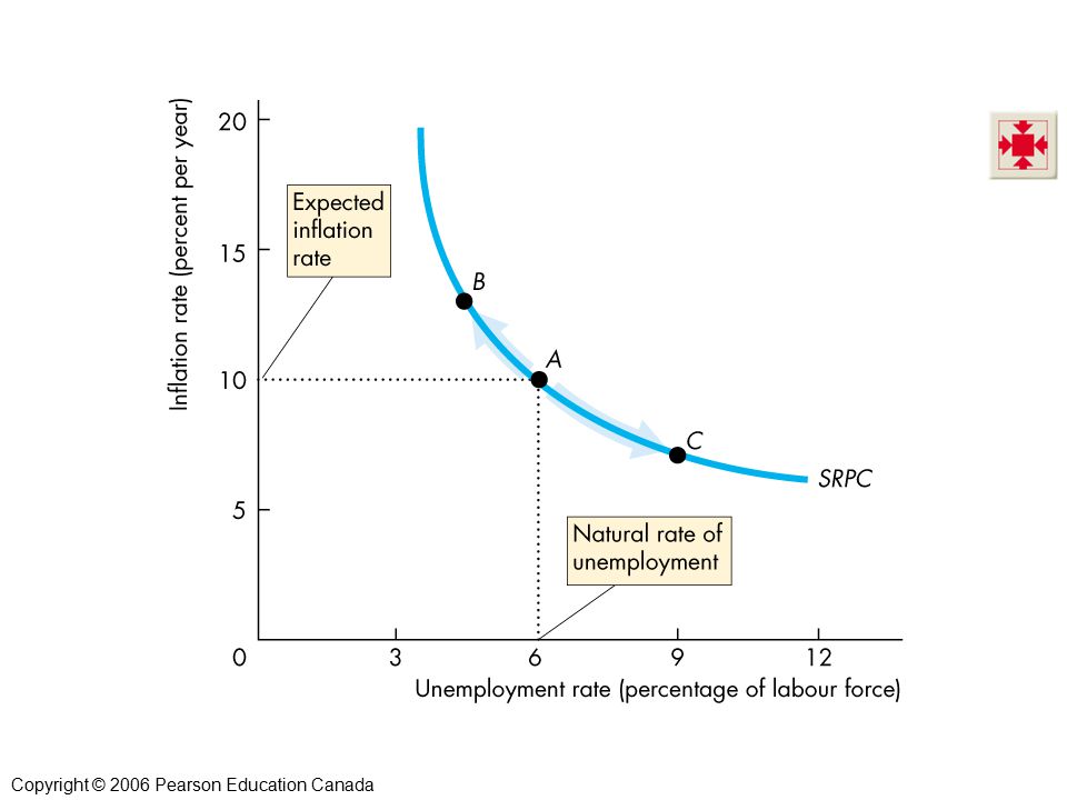
Figure illustrates a short-run Phillips curve (SRPC)—a downward-sloping curve. If the unemployment rate falls, the inflation rate rises. And if the unemployment rate rises, the inflation rate falls.

The negative relationship between the inflation rate and unemployment rate is explained by the AS-AD model. Figure shows how. Students can become confused about the tie between the Phillips curve and the AS-AD model. Although this relationship is nicely developed in the text, some students will remain baffled. I do not think that a principles course is the appropriate place to derive the link between the two in much detail. Point out that the vertical long-run aggregate supply curve is analogous to the vertical long-run Phillips curve. The point that the long-run aggregate supply curve is vertical means that a higher price level has no effect on real GDP and hence no effect on the unemployment rate. Similarly, the fact that the long-run Phillips curve is vertical implies that a higher inflation rate has no effect on the unemployment rate and hence no effect on real GDP. The analogy also carries over to the short-run curves: the positively sloped short-run aggregate supply curve shows that in the short-run an unexpected higher price level raises real GDP and thus lowers unemployment. In the same way, the negatively sloped short-run Phillips curve demonstrates that in the short-run an unexpected higher inflation rate lowers unemployment, thereby raising real GDP. Students find that the two diagrams complement each other. The bottom line is that the two models tell the same story: AS-AD focuses on P and Y and the Phillips curve focuses on inflation and unemployment.

Aggregate demand is expected to increase to AD1 so the money wage rate rises and the short-run aggregate supply curve shifts to SAS1. If this outcome occurs, the inflation rate is 10 percent and unemployment is at the natural rate.

An unexpectedly large increase in aggregate demand raises the inflation rate and increases real GDP, which lowers the unemployment rate. A higher inflation is associated with a lower unemployment, as shown by a movement along a short-run Phillips curve.

An unexpectedly small increase in aggregate demand lowers the inflation rate and decreases real GDP, which raises the unemployment rate. A lower inflation is associated with a higher unemployment, as shown by a movement along a short-run Phillips curve.

The Long-Run Phillips Curve The long-run Phillips curve shows the relationship between inflation and unemployment when the actual inflation rate equals the expected inflation rate.

Figure illustrates the long-run Phillips curve (LRPC) which is vertical at the natural rate of unemployment. Along the long-run Phillips curve, because a change in the inflation rate is anticipated, it has no effect on the unemployment rate.

Figure also shows how the short-run Phillips curve shifts when the expected inflation rate changes. When expected inflation falls from 10 percent to 7 percent, the short-run Phillips curve shifts downward by an amount equal to the fall in the expected inflation rate.

But with an expected inflation rate of 10 percent a year, a fall in the actual inflation rate to 7 percent a year would increase the unemployment rate to 9 percent at point C.

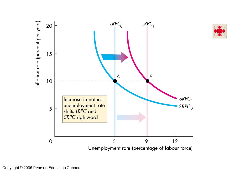
Changes in the Natural Unemployment Rate A change in the natural unemployment rate shifts both the long-run and short-run Phillips curves. Figure illustrates.

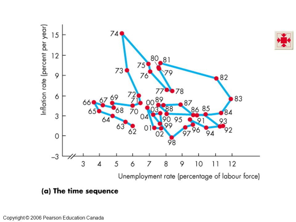
The Canadian Phillips Curve Each dot represents the combination of inflation and unemployment in a particular year in Canada.

Figure (a) shows the actual path traced out in inflation rate-unemployment rate space.

Figure 27.14(b) interprets the data with shifting short-run and long-run Phillips curves.

In the 1960s, the natural rate of unemployment was 5 percent, so the long-run Phillips curve was LRPC1. With an expected inflation rate of 3 percent a year, the short-run Phillips curve was SRPC1.

During the 1970s and through 1982, the natural rate of unemployment increased to 10 percent. The long-run Phillips curve shifted to LRPC2. The expected inflation increased to 9 percent a year, and the short-run Phillips curve shifted to SRPC2.

During the 1980s and 1990s, the natural rate of unemployment decreased to 7 percent. The long-run Phillips curve shifted to LRPC3. The expected inflation rate fell to 2 percent a year and the short-run Phillips curve shifted back to SRPC1.

Interest Rates and Inflation
Interest rates and inflation rates are correlated, although they differ around the world. Figure 27.15(a) shows a positive correlation between the inflation rate and the nominal interest rate over time in Canada. This section has two main purposes: to reinforce that real interest rates and nominal interest rates are determined in wholly different ways, and then to remind students of the link between them via anticipated inflation. This is also a place where one can again show why and how short-term and long-term interest rates can and do diverge, and how even short-term real interest rates can differ between countries because of differences in perceived risk. With respect to short-term rates, this is mostly exchange risk, but that point does not need to be emphasized at this point. Using Web sites or newspapers, find the short-term interest rates and current inflation rates of some countries, including not only nice stable ones (U.S., Canada, UK, Germany, Switzerland, Japan) but a few that students, at least, will view as unstable and risky (e.g. South Africa, Russia, Brazil, Argentina, Indonesia). This will show that although differences in inflation explain part of the differences, there are also differences in real interest rates that arise from differences in risk perceptions. This can generate a useful discussion if you then ask students whether that might imply that there are potential investments in the “risky” countries that have higher expected rates of return than all investments undertaken in the “stable” countries.

Figure 27.15(b) shows a positive correlation between the inflation rate and the nominal interest rate across countries.

How Interest Rates are Determined The real interest rate is determined by investment demand and saving supply in the global capital market. The real interest rate adjusts to make the quantity of investment equal the quantity of saving. National real rates vary because of differences in risk. The nominal interest rate is determined by the demand for money and the supply of money in each nation’s money market.

Why Inflation Influences the Nominal Interest Rate On the average, and other things remaining the same, a 1 percentage point rise in the inflation rate leads to a 1 percentage point rise in the nominal interest rate. Why? The answer is that the financial capital market and the money market are closely interconnected. The investment, saving, and demand for money decisions that people make are connected and the result is that equilibrium nominal interest rate approximately equals the real interest rate plus the expected inflation rate. That is, inflation influences the nominal interest rate to maintain an equilibrium real interest rate.

27 Inflation CHAPTER Notes and teaching tips: 4, 8, 17, 28, 36, 37, 52, 56, and 78. To view a full-screen figure during a class, click the red “expand”

Similar presentations

Presentation on theme: "27 Inflation CHAPTER Notes and teaching tips: 4, 8, 17, 28, 36, 37, 52, 56, and 78. To view a full-screen figure during a class, click the red “expand”"— Presentation transcript:

Similar presentations

About project

Feedback

Log in

Auth with social network:

27 Inflation CHAPTER Notes and teaching tips: 4, 8, 17, 28, 36, 37, 52, 56, and 78. To view a full-screen figure during a class, click the red “expand”

Similar presentations

Presentation on theme: "27 Inflation CHAPTER Notes and teaching tips: 4, 8, 17, 28, 36, 37, 52, 56, and 78. To view a full-screen figure during a class, click the red “expand”"— Presentation transcript:

Similar presentations

About project

Feedback