1. University of Minnesota
Extreme Events, Heavy Tails, and
the Generating Processes:
Examples from Hydrology and Geomorphology
Efi Foufoula-Georgiou
SAFL, NCED
University of Minnesota
E2C2 – GIACS Advanced School on “Extreme Events: Nonlinear Dynamics and Time Series Analysis
Comorova, Romania
September 3-11, 2007

2. Underlying Theme
In Hydrology and Geomorphology “Fluctuations” around the mean behavior are of high magnitude.
Understanding their statistical behavior is useful for prediction of extremes and also for understanding spatio-temporal heterogeneities which are hallmarks of the underlying process- generating mechanism.
These fluctuations are often found to exhibit power law tails and scaling

3. PRESENCE OF SCALING
... scaling laws never appear by accident. They always manifest a property of the phenomenon of basic importance … This behavior should be discovered, if it exists, and its absence should also be recognized.”
Barenblatt (2003)

4. High-resolution temporal rainfall data
(courtesy, Iowa Institute of Hydraulic Research – IIHR)
~ 5 hrs
t = 10s
~ 1 hr
t = 5s
If easy we could add inside the red box approx 5 hours and underneath Dt= 10 secs and in the green box approx 1 hour and underneath Dt=5 secs
DONE

5. Noyo River basin

6. Sediment accumulation series Time series of bed elevation
STREAMLAB 2006
Data Available:
Sediment accumulation series
Time series of bed elevation
Laser transects of bed elevation
Pan-1
Pan-2
Pan-3
Pan-4
Pan-5

7. Experimental setup Data Available: Sediment accumulation series
Time series of bed elevation
Laser transects of bed elevation
D50 = 11.3mm
Pan-1
Pan-2
Pan-3
Pan-4
Pan-5
Discharge controlled here
Channel Width = 2.75 m
Channel Depth = 1.8 m
D50=11.3 mm
1.0
Diameter [mm]
100
Discharge capacity: 8500 lps
Coarse sediment recirculation system located 55 m from upstream end.

8. Bed Elevation

9. Sediment Transport Rates
Accumulated series (Sc(t))
Nearest neighbor differences (S(t))

10. SEDIMENT FLUX: VARIABILITY AT ALL SCALES
Sc (t) = Accumulated sediment over an interval of 0 to t sec

11. Noise-free sediment transport rates
Weigh pan bedload transport rates (Q = 5.5 m3/s) (a) 1 s averaging and 0 point skip
(b) 15s averaging time and 6 point skip (from Ramooz and Rennie, 2007)

12. Background
In Hydrology and Geomorphology “Fluctuations” around the mean behavior are of high magnitude.
Understanding their statistical behavior is useful for prediction of extremes and also for understanding spatio-temporal heterogeneities which are hallmarks of the underlying process- generating mechanism.
These fluctuations are often found to exhibit power law tails and scaling
There is a continuous need for new mathematical tools of analysis and new paradigms of modeling physical phenomena that exhibit a rich statistical structure

13. Localized Scaling Analysis: Multifractal Formalism
• Characterize a signal f(x) in terms of its local singularities
h=0.3
h=0.7
Ex: h(x0) = 0.3 implies f(x) is very rough around x0.
h(x0) = 0.7 implies a “smoother” function around xo.

14. Multifractal Formalism
• Spectrum of singularities D(h)
D(h) h
• D(h) can be estimated from the statistical moments of the fluctuations.
Legendre Transform

15. Multifractal Spectra
• Spectrum of scaling exponents t(q) and Spectrum of singlularities D(h)
monofractal h
multifractal h

16. Spectrum of singularities
Multifractal Spectra
Spectrum of scaling exponents
Spectrum of singularities
D(h) -1 1 2 3 4 5 6 7
(2)
Slopes (q) q Df
Please add the symbol D_f, <h> horizontal axis h, hmin/hmax and possibly an arrow to show that the derivative is taken at that point (as in paper)
DONE h
hmin
hmax

17. Wavelet-based multifractal formalism (Muzy et al., 1993; Arneodo et al., 1995)
CWT of f(x) :
The local singularity of f(x) at point x0 can be characterized by the behavior of the wavelet coefficients as they change with scale, provided that the order of the analyzing wavelet n > h(x0)
Can obtain robust estimates of h(x0) using “maxima lines” only: Ta(x) i.e. WTMM
In definition of wavelet either correct f(u) inside the integral or replace location with x_o and have the running variable as x
This is strange.. I thought I fixed this the very first time I sent you.
Same thing here, I fixed it, and now the font changes. I suspect Roshan uses a different equation editor (probably a better one) than I do.
It can be shown that

18. (direct access to statistics of singularities)
f(x)
Structure Function
Moments of
|f(x+l) – f(x)|
T[f](x,a)
Partition Function
Moments of
|T[f](x,a)|
 Partition Function
Moments of |Ta(x)|
(access to q < 0)
 Cumulant analysis
Moments of ln |Ta(x)|
(direct access to statistics of singularities)
WTMM Ta(x)

19. Two Examples Landscape dissection
Planform topology of channelized and unchannelized paths (branching structure of river networks and hillslope drainage patterns)
Vertical structure of landform heterogeneity perpendicular to the river paths.
River bedform morphodynamics and sediment transport rates

20. Two Ways of Looking at Landscapes
Planform Dissection
Topology of the river network (channelized paths): W(x)
Topology of the unchannelized flow paths: A(x) $ W(x)
Vertical “roughness” of topography
Structure of the “river corridor width” (RCW) series

21. Width and Area Functions of a River Network
# of channels intersected by a contour of equal flow length to the outlet
# of pixels of equal flow length to the outlet
Topology of river network
Topology of the hillslope drainage paths and topology of river network

22. Width and Area Functions of a River Network
# of channels intersected by a contour of equal flow length to the outlet
# of pixels of equal flow length to the outlet
Topology of river network
Topology of the hillslope drainage paths and topology of river network

23. Area and Width Functions
Walawe River, Sri Lanka
(90x90m)
A;2,000 km2

24. Area and Width Functions
Noyo River Basin, California, USA
(10x10m)
A;143 km2

25. Walawe River Basin: deviation from simple scaling
A(x)
W(x)
W(x)
A(x)
A rich multifractal structure is observed which is different for A(x) and W(x)

26. Noyo River Basin: deviation from simple scaling
A(x)
W(x)
A rich multifractal structure is observed which is different for A(x) and W(x)

27. Noyo River Basin (10x10m; A;143 km2)
c1 ; c2 = SR = km
“Hillslope” path dominated
“smoother” overall than W(x)
Hillslope drainage dissection is s-s between scales 0.1 km – 0.5km
Statistics of the density of hillslope drainage paths strongly depend on scale
c1 ; c2 ; SR = 0.13 – 0.70 km
River network path dominated
“Rougher “overall” than A(x)
Channel network landscape dissection is s-s between scales 0.1 km to 0.7 km
Strong inntermittency (higher moments of pdf of channel drainage density has a strong dependence on scale)
Pay attention not only to the average properties of landscape dissection but to higher moments

28. Walawe River Basin (90x90m; A;2,000 km2)
c1 ; c2 = SR = km
c1 ; c2 ; SR = km
Accurate characterization of higher moments needs high resolution topography data

29. Real River Networks C1=0.77 C2=0.11 C1=0.40 C2=0.05 C1=0.80 C2=0.05
Noyo River basin, CA
(10x10m)
A;1430 km2
Walawe River, Sri Lanka
(90x90m)
A;2,000 km2
South Fork Eel River, CA
(1x1m & 10x10m)
A;154 km2
C1=0.77
C2=0.11
C1=0.40
C2=0.05
C1=0.80
C2=0.05
A(x)

30. Area Functions of Simulated Trees
Peano Basin
Not comparable to real networks
Shreve’s random
network model
c1=0.5
c2=0
Stochastic S-S model with (a , b)=(1 , 2)
c1=0.62
c2=0

31. Important Observation: The effect of higher order statistical moments
(a,b)=(1,2) ® Tk correspond to those of Shreve model.
Shreve Model H ; 0.5
S-S tree H ; 0.62
Yet: ß
Difference reflects the effect of the statistical distribution of Tk (Tk: Deterministic for Shreve’s model; Poisson distributed for S-S tree) ß
Randomness in the River Network Topology is reflected in the statistical properties of the width function

32. Conclusions on topology of drainage paths
Simulated river networks show different multifractal properties than real river networks. [s-s trees are monofractal with H = 0.5 – 0.65 while real networks are multifractal with H ; 0.4 – 0.8].
Differences between scaling properties of A(x) and W(x) depict differences in the branching topology of channelized vs. unchannelized drainage paths.
Deviation from monoscaling stresses the importance of the dependence on scale of higher order statistics of the branching structure.

33. Implications for Network Hydrology?
W(x) = # of channels intersected by a contour of equal length x to the outlet |W(x+dx)-W(x)| = # of new channels within a strip of dx flow distance to outlet = # of copies of new hillslope hydrographs combined in phase and delivered to channel.
Shreve’s random topology model: c1=0.5, c2=0.0, for all dx
Walawe River Basin: c1=0.5, c2=0.13 for dx =2 – 6 km
Deviation from scale invariance (c2 ¹ 0) Þ extended S-S within a limited range of scales
An intermittent application of in-phase new hillslope hydrographs along the river network Þ Higher chance of a disproportionately larger # of in-phase new hydrographs to enter the network at smaller than larger distances apart Þ Implications for routing (e.g., scale-dependent convolution? geomorphologic dispersion?) Þ Implications for scaling of hydrographs?

34. Implications for Network Hydrology?
Conjecture: Deviation from scale invariance in W(x), implies that the variability of the in-phase hillslope hydrographs entering the network depends on “scale”
ÞImplications for routing? scale-dependent convolution? geomorphologic dispersion?
Þ Implications for scaling of hydrographs?

35. River Corridor Width Functions

36. River Corridor Width Function (D=5m)

37. SCALING OR NOT?
“Why are scaling laws of such distinguished importance?
The answer is that scaling laws never appear by accident. They always manifest a property of the phenomenon of basic importance … This behavior should be discovered, if it exists, and its absence should also be recognized.”
Barenblatt (2003)

38. Specific Questions: Area and Width Functions
Does the topology of river networks leave a unique signature on the scaling of W(x) and A(x)?
How different are the scaling properties of commonly used simulated trees and those of real river networks?
Are there differences between the scaling properties of A(x) and W(x) and what do these tell us about the topology of hillslope vs. channelized drainage patterns in a river basin?
What are the hydrological implications of the above?

39. Statistical multiscaling: beyond global analysis
Need a localized multiscale analysis methodology to locally characterize abrupt fluctuations (coming about from the underlying branching topology)
“Energy” associated with the “small scales” is not uniformly distributed over the river network ® characterize the statistical nature of the points (flow distances from outlet) at which abrupt local changes in W(x) or A(x) exist.
The multifractal formalism (Parisi and Frisch, 1985) allows this characterization from the statistics of W(x) and A(x) “fluctuations.”

40. Multifractal Formalism
• Spectrum of singularities D(h)
D(h) h
• D(h) can be estimated from the statistical moments of the fluctuations.
Legendre Transform

41. Multifractal Spectra
• Spectrum of scaling exponents t(q) and Spectrum of singlularities D(h)
monofractal h
multifractal h

42. Walawe River Basin: deviation from simple scaling
A(x)
W(x)
W(x)
A(x)
A rich multifractal structure is observed which is different for A(x) and W(x)

43. Noyo River Basin: deviation from simple scaling
A(x)
W(x)
A rich multifractal structure is observed which is different for A(x) and W(x)

44. Noyo River Basin (10x10m; A;143 km2)
c1 ; c2 = SR = km
“Hillslope” path dominated
“smoother” overall than W(x)
Hillslope drainage dissection is s-s between scales 0.1 km – 0.5km
Statistics of the density of hillslope drainage paths strongly depend on scale
c1 ; c2 ; SR = 0.13 – 0.70 km
River network path dominated
“Rougher “overall” than A(x)
Channel network landscape dissection is s-s between scales 0.1 km to 0.7 km
Strong inntermittency (higher moments of pdf of channel drainage density has a strong dependence on scale)
Pay attention not only to the average properties of landscape dissection but to higher moments

45. Walawe River Basin (90x90m; A;2,000 km2)
c1 ; c2 = SR = km
“Hillslope” path dominated
“rougher” overall than W(x)
Hillslope drainage dissection is s-s between scales 0.4 km – 3.0 km
Statistics of the density of hillslope drainage paths depends on scale
c1 ; c2 ; SR = km
River network path dominated
Smoother “overall” than A(x)
Channel network landscape dissection is s-s between scales 2.6 km to 6.0 km
Much more intermittent (higher moments of pdf of channel drainage density has a strong dependence on scale)
Accurate characterization of higher moments needs high resolution topography data

46. Implications for Network Hydrology?
Conjecture: Deviation from scale invariance in W(x), implies that the variability of the in-phase hillslope hydrographs entering the network depends on “scale”
ÞImplications for routing? scale-dependent convolution? geomorphologic dispersion?
Þ Implications for scaling of hydrographs?

47. Real River Networks C1=0.77 C2=0.11 C1=0.40 C2=0.05 C1=0.80 C2=0.05
Noyo River basin, CA
(10x10m)
A;1430 km2
Walawe River, Sri Lanka
(90x90m)
A;2,000 km2
South Fork Eel River, CA
(1x1m & 10x10m)
A;154 km2
C1=0.77
C2=0.11
C1=0.40
C2=0.05
C1=0.80
C2=0.05
A(x)

48. Noyo River basin

49. Area Functions of Simulated Trees
Peano Basin
Not comparable to real networks
Shreve’s random
network model
c1=0.5
c2=0
Stochastic S-S model with (a , b)=(1 , 2)
c1=0.62
c2=0

50. Stochastic S-S Trees
(Tokunaga, 1996, 1978; Peckham, 1995) •
= average # of tributaries of order w¢ that branch into a stream of order w

51. Stochastic S-S Network Model: Area Function
(a , b)
(0.75, 1.894)
(1, 2)
(1.25, 2.095)
(1.5, 2.183)
(1.75, 2.266)
(1.5, 2.5)
(1, 3) D 2
1.76
1.41
order 13 12 11 10
3894
4160
3618
5817
3950
6435
14827 c1
0.65
0.62
0.55 c2
0.00
0.01
Note: as a increases, c1 decreases, i.e., when “branching rate” increases; A(x) exhibits wilder fluctuations and becomes more irregular.

52. Important Observation: The effect of higher order statistical moments
(a,b)=(1,2) ® Tk correspond to those of Shreve model.
Shreve Model H ; 0.5
S-S tree H ; 0.62
Yet: ß
Difference reflects the effect of the statistical distribution of Tk (Tk: Deterministic for Shreve’s model; Poisson distributed for S-S tree) ß
Randomness in the River Network Topology is reflected in the statistical properties of the width function

53. A(x) W(x) Walawe: A;2,000 km2 (90x90m) c1=0.37 – 0.40 c2=0.05 c1;0.50
South Fork: A;154 km2 (1x1m & 10x10m)
c1=0.80
Beaver Creek: A;622 km2 (30x30m)
c1=0.44
Noyo River Basin: A; 143 km2 (1x1m)
c1=0.77
c2=0.11
c1=0.46
Lower Noyo River Basin: A; km2 (1x1m)
c1=
c2=

54. Conclusions on topology of drainage paths
Simulated river networks show different multifractal properties than real river networks. [s-s trees are monofractal with H = 0.5 – 0.65 while real networks are multifractal with H ; 0.4 – 0.8].
Differences between scaling properties of A(x) and W(x) depict differences in the branching topology of channelized vs. unchannelized drainage paths.
Deviation from monoscaling stresses the importance of the dependence on scale of higher order statistics of the branching structure.

55. Implications for Network Hydrology?
W(x) = # of channels intersected by a contour of equal length x to the outlet |W(x+dx)-W(x)| = # of new channels within a strip of dx flow distance to outlet = # of copies of new hillslope hydrographs combined in phase and delivered to channel.
Shreve’s random topology model: c1=0.5, c2=0.0, for all dx
Walawe River Basin: c1=0.5, c2=0.13 for dx =2 – 6 km
Deviation from scale invariance (c2 ¹ 0) Þ extended S-S within a limited range of scales
An intermittent application of in-phase new hillslope hydrographs along the river network Þ Higher chance of a disproportionately larger # of in-phase new hydrographs to enter the network at smaller than larger distances apart Þ Implications for routing (e.g., scale-dependent convolution? geomorphologic dispersion?) Þ Implications for scaling of hydrographs?

56. Implications for Network Hydrology?
Conjecture: Deviation from scale invariance in W(x), implies that the variability of the in-phase hillslope hydrographs entering the network depends on “scale”
ÞImplications for routing? scale-dependent convolution? geomorphologic dispersion?
Þ Implications for scaling of hydrographs?

57. South Fork Eel River, CA
Area = 351 km2

58. River Corridor Width Function (D=5m)

59. Questions What is the statistical structure of RCW(x)?
Do physically distinct regimes exhibit statistically distinct signatures?
How can the statistical structure be used in modeling and prediction of hydrographs, sedimentographs and pollutographs across scales?

60. SOUTH FORK EEL RIVER, CA: Hypsometric Profile

61. River Reach: 0-6 Km

62. Reach: km
Right
Left

63. Motivating questions
Are statistically-distinct regimes the result of physically-distinct valley- forming processes?
Do differences in mechanistic laws governing valley-forming processes leave their signature on the statistical properties of valley geometry?
How can these statistical properties be used for modeling and prediction?

64. River Corridor Width Function: South Fork Eel River
6 km
14 km
20 km
28 km
35 km
89 tributaries: (1 km2 – 150 km2)

65. River Reach: 0-6 km

66. River Reach: km

67. Recall the interpretation of multifractal parameters
C1: a larger value means a smoother function (more smoothing than roughening mechanisms are responsible for the formation of this surface)
C2: a larger value means more intermittency (localized very large fluctuations or “bursts” are present signaling nonlinear and localized transport mechanisms)

68. SUMMARY OF RESULTS
Right-Left asymmetry

69. INTERPRETATION OF RESULTS
More localized NL transport mechanism?
More localized on L than R side?
Smoother overall valleys?
Presence of more terraces in R than L?

70. Conclusions on RCW Series
RCW fluctuations exhibit a deviation from scale-invariance
As we move from the bedrock to more alluvial valleys, the statistical intermittency increases indicating an increased presence of very localized abrupt fluctuations probably due to increasingly localized transport mechanisms.
There is a significant left-right asymmetry in the statistical structure of RCWs reflecting different underlying processes in each side of the river.

71. Conclusions and Open Questions…
Hillslope “roughness” seems to carry the signature of valley forming processes; need to provide a complete hierarchical characterization. Do hillslope evolution models reproduce this structure? What is the effect on hillslope sediment variability of the higher order statistics of travel paths to streams?

72. Some Words of Caution
There exist multiple ways by which an emergent pattern can manifest itself from mechanistic or physical processes:
Ex. 1:
Omittance of floodplain and two distinct rainfall regimes
-or- channel-floodplain interactions with a single rainfall regime ß
Both can give a scaling break in floods Þ need enough underlying observations to pose the right hypotheses which might be region-dependent
Ex. 2:
Peano basins have been used in modeling studies to relate the scaling of hydrograph peaks to the scaling of the peaks of the width functions and several runoff production mechanisms.
But scaling of Peano basin W(x) ¹ scaling of real network W(x) Þ Implications?

73. References
Gangodagamage, C., E. Barnes, and E. Foufoula-Georgiou, Scaling in river corridor widths depicts organization in valley morphology, Geomorphology, doi: /j.geomorph , 2007.
Lashermes, B. and E. Foufoula-Georgiou, Area and width functions of river networks: new results on multifractal properties, Water Resources Research, doi: /2006WR005329, 2007
Lashermes, B., E. Foufoula-Georgiou, and W. Dietrich, Channel network extraction from high resolution topograhy using wavelets, Geophysical Research Letters, in press, 2007.
Sklar L. S., W. E. Dietrich, E. Foufoula-Georgiou, B. Lashermes, D. Bellugi, Do gravel bed river size distributions record channel network structure?, Water Resources Research, 42, W06D18, doi: /2006WR005035, 2006.
Barnes, E. M.E. Power, E. Foufoula-Georgiou, M. Hondzo, and W.E. Dietrich, Scaling Nostic biomass in a gravel-bedrock river: Combining local dimensional analysis with hydrogeomorphic scaling laws, Geophysical Research Letters, under review.

74. Experimental setup Data Available: Sediment accumulation series
Time series of bed elevation
Laser transects of bed elevation
D50 = 11.3mm
Pan-1
Pan-2
Pan-3
Pan-4
Pan-5
Discharge controlled here
Channel Width = 2.75 m
Channel Depth = 1.8 m
D50=11.3 mm
1.0
Diameter [mm]
100
Discharge capacity: 8500 lps
Coarse sediment recirculation system located 55 m from upstream end.

75. Sediment accumulation series Time series of bed elevation
STREAMLAB 2006
Data Available:
Sediment accumulation series
Time series of bed elevation
Laser transects of bed elevation
Pan-1
Pan-2
Pan-3
Pan-4
Pan-5

76. QUESTIONS
Do the statistics of sediment transport rates depend on “scale” (sampling interval or time interval of averaging) and how?
Does this statistical scale-dependence depend on flow rate, bed shear stress, and bedload size distribution (e.g., gravel vs. sand, etc.)
Do the statistics of sediment transport relate to the statistics of bedform morphodynamics and how?
What are the practical implications of all these?

77. Sediment Transport Rates
Accumulated series (Sc(t))
Nearest neighbor differences (S(t))

78. VARIABILITY AT ALL SCALES
Sc (t) = Accumulated sediment over an interval of 0 to t sec

79. Noise-free sediment transport rates
Weigh pan bedload transport rates (Q = 5.5 m3/s) (a) 1 s averaging and 0 point skip
(b) 15s averaging time and 6 point skip (from Ramooz and Rennie, 2007)

80. LOCAL “ROUGHNESS” OF A SIGNAL
Characterize a signal f(x) in terms of its local singularities
Ex: h(x0) = 0.3 implies f(x) is very rough around x0.
h(x0) = 0.7 implies a “smoother” function around xo.

81. MULTIFRACTAL FORMALISM
• Spectrum of singularities D(h)
D(h) h
• D(h) can be estimated from the statistical moments of the fluctuations.
Legendre Transform

82. MULTIFRACTAL FORMALISM
• Spectrum of scaling exponents t(q)
monofractal h
multifractal h

83. ANALYSIS METHODOLOGY: ADVANTAGES
Local analysis (as opposed to global, e.g., spectral analysis)
Can characterize the statistical structure of localized abrupt fluctuations over a range of scales
Wavelet-based multifractal formalism -- uses generalized fluctuations instead of standard differences (f(x) – f(x+dx))
Can automatically remove non-stationarities in the signal both in terms of overall trends and in terms of low-frequency oscillations coming from dune or ripple effects
Can automatically remove noise in the signals and point to the minimum scale that can be safely interpreted
Can characterize effectively how pdfs change with scale with only one or two parameters

84. SEDIMENT TRANSPORT RATES: Q = 5500 lps
log2
Noise
Variability levels off
Scaling range
C1=1.10
C2=0.10
15 min
1 min

85. Q = 4300 lps Noise C1=0.55 C2=0.15 Scaling range
log2
Noise
C1=0.55
C2=0.15
Scaling range
Statistical Variability regime changes
1 min
10 min

86. SEDIMENT TRANSPORT RATES: SUMMARY TABLE OF c1, c2
Polynomial approx.
Q (lps)
Pan
Scaling Range
(min)
Shield stress
τ(2) –
2 τ(1) c1 c2
c1 (cumulants) 2
1 – 10
0.085
-0.26
0.40
0.15
0.53
4300 3
-0.20
0.56
0.14
0.57 4
1 -- 3
-0.10
0.52
0.05
2 – 15
0.111
-0.12
1.30
0.11
1.34
4900
-0.14
1.33
0.10
-0.09
1.24
0.08
1 – 15
0.196
-0.13
1.09
0.09
1.17
5500
-0.15
1.07
1.18
1.15
1.25

87. Higher c1 means a “smoother” signal
RECALL
Higher c1 means a “smoother” signal
Higher c2 means a stronger dependence of the higher moments on scale, spatially inhomogeneous distribution of extreme bursts, more likelihood of extreme bursts at very small scales
• c2=0 monofractal ® t(2)=2t(1)
• all moments can be scaled with one parameter c1=H only
• CV is constant with scale
• c2¹0 multifractalfractal ® t(2)<2t(1)
• need 2 parameters c1, c2 to scale pdfs
• CV decreases with increase in scale

88. INTERPETATION AND PRACTICAL IMPLICATIONS
Low flows:
The sedimentation rate is a “fractal” (s-s) process
The longer the time interval, the lower the average sedimentation rate (in double the time, sedimentation rate decreases by a factor of 0.7 = 2**(-0.4))
The smaller the time interval, the higher the chance to encounter an extreme localized rate
High Flows:
The change in sedimentation rate is a “fractal” (s-s) process
The longer the time interval, the higher the expected change in sedimentation rate (in double the time, the gradient of sedimentation rate changes by a factor of 1.1 = 2**(0.2))

89. Bed Elevation

90. Bed elevation data
Note: these series are plotted till 3000 data points to show the same scale

91. BED ELEVATION TEMPORAL SERIES: Q = 5500 lps
Scaling range
C1=0.70
C2=0.11
0.5 min
8 min

92. BED ELEVATION TEMPORAL SERIES: Q = 4300 lps
Scaling range
C1=0.55
C2=0.05
1 min
12 min

93. Inferences on Nonlinearity
Basu and Foufoula-Georgiou, Detection of nonlinearity and chaoticity in time series using the transportation distance function, Phys. Letters A, 2002.

94. Finite Size Lyapunov Exponent (FSLE)
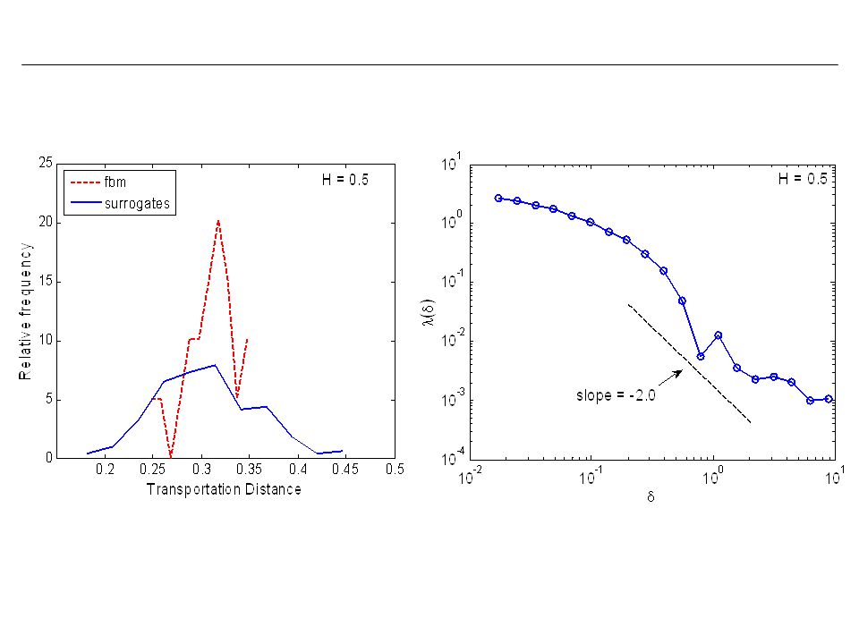
FSLE is based on the idea of error growing time (Tr(d)), which is the time it takes
for a perturbation of initial size δ to grow by a factor r (equals to √2 in this work)
measure the typical rate of exponential divergence of nearby trajectory
δ(nr) size of the perturbation at the time nr at which this perturbation first exceeds (or becomes equal to) the size rδ
For an initial error δ and a given tolerance ∆ = rδ, the average predictability time
Basu et al., Predictability of atmospherci boundary layer flows as a function of scale, Geophys. Res. Letters, 2002.

97. CONCLUDING REMARKS
Documented a clear dependence of sediment transport rates and of the corresponding bed elevation series on “scale”
Need to explore more rigorously the dependence on flow rate, grain size distribution, etc. and how the self-organized structure of the bed elevation reflects itself in the statistics of the sediment transport rate
Must think about the implications of scaling for sampling and also for the development of sediment transport equations

98. References
Gangodagamage, C., E. Barnes, and E. Foufoula-Georgiou, Scaling in river corridor widths depicts organization in valley morphology, Geomorphology, doi: /j.geomorph , 2007.
Lashermes, B. and E. Foufoula-Georgiou, Area and width functions of river networks: new results on multifractal properties, Water Resources Research, doi: /2006WR005329, 2007
Lashermes, B., E. Foufoula-Georgiou, and W. Dietrich, Channel network extraction from high resolution topograhy using wavelets, Geophysical Research Letters, in press, 2007.
Sklar L. S., W. E. Dietrich, E. Foufoula-Georgiou, B. Lashermes, D. Bellugi, Do gravel bed river size distributions record channel network structure?, Water Resources Research, 42, W06D18, doi: /2006WR005035, 2006.
Barnes, E. M.E. Power, E. Foufoula-Georgiou, M. Hondzo, and W.E. Dietrich, Scaling Nostic biomass in a gravel-bedrock river: Combining local dimensional analysis with hydrogeomorphic scaling laws, Geophysical Research Letters, under review.

99. THE END

102. Transportation Distance
based on both the geometric and probabilistic aspects of point distributions
provide a measure of long term qualitative differences between any
two time series (x and y).
μij > 0 amount of material shipped from box Bi to box Bj
δij taxi cab metric normalized to the embedding dimension between the centres of Bi and Bj

103. 4300 4900 5500 Bed elevation Summary Table 2 4 1-12 0.085 -0.0396
Polynomial approx.
Q (lps)
Probe
Scaling Range
(min)
Shield stress
τ(2) -2* τ(1) c1 c2
c1 (cumul)
4300 4
1-12
0.085
0.5686
0.0488
0.5546
4900 3
0.5-20
0.111
0.6187
0.0658
0.5784
5500
0.5-8
0.196
0.7054
0.1169
0.7523
RESULT: The higher the flow, the smoother the bed elevation fluctuations overall
(larger c1) but the higher chance to find localized rough spots inhomogeneously
distributed over time (c2 higher)

104. RECALL 1.
Dx(k ×Dt) = Sediment transported during a time period k ×Dt
Dt = Sampling interval ~
• c2=0 monofractal ® t(2)=2t(1)
• all moments can be scaled with one parameter c1=H only
• CV is constant with scale 2.
• c2¹0 multifractalfractal ® t(2)<2t(1)
• need 2 parameters c1, c2 to scale pdfs
• CV decreases with increase in scale

105. High-resolution temporal rainfall data
(courtesy, Iowa Institute of Hydraulic Research – IIHR)
~ 5 hrs
t = 10s
~ 1 hr
t = 5s
If easy we could add inside the red box approx 5 hours and underneath Dt= 10 secs and in the green box approx 1 hour and underneath Dt=5 secs
DONE