1. Fi8000 Optimal Risky Portfolios Milind Shrikhande

2. Investment Strategies ☺ Lending vs. Borrowing (risk-free asset) ☺ Lending: a positive proportion is invested in the risk-free asset (cash outflow in the present: CF 0 0) ☺ Borrowing: a negative proportion is invested in the risk-free asset (cash inflow in the present: CF 0 > 0, and cash outflow in the future: CF 1 0, and cash outflow in the future: CF 1 < 0)

3. Lending vs. Borrowing rf C A B A Lend Borrow

4. Investment Strategies ☺ A Long vs. Short position in the risky asset ☺ Long: A positive proportion is invested in the risky asset (cash outflow in the present: CF 0 0) ☺ Short: A negative proportion is invested in the risky asset (cash inflow in the present: CF 0 > 0, and cash outflow in the future: CF 1 0, and cash outflow in the future: CF 1 < 0)

5. Long vs. Short STD(R) E(R) B A Long A and Short B Long A and Long B Short A and Long B

6. Investment Strategies ☺ Passive risk reduction: The risk of the portfolio is reduced if we invest a larger proportion in the risk-free asset relative to the risky one ☺ The perfect hedge: The risk of asset A is offset (can be reduced to zero) by forming a portfolio with a risky asset B, such that ρ AB =(-1) ☺ Diversification: The risk is reduced if we form a portfolio of at least two risky assets A and B, such that ρ AB <(+1) The risk is reduced if we add more risky assets to our portfolio, such that ρ ij <(+1)

7. One Risky Fund and one Risk-free Asset: Passive Risk Reduction rf C A B A Reduction in portfolio risk Increase of portfolio Risk

8. Two Risky Assets with ρ AB =(-1): The Perfect Hedge STD(R) E(R) B A Minimum Variance is zero P min

9. The Perfect Hedge – an Example What is the minimum variance portfolio if we assume that μ A =10%; μ B =5%; σ A =12%; σ B =6% and ρ AB =(- 1) ?

10. The Perfect Hedge – Continued What is the expected return μ min and the standard deviation of the return σ min of that portfolio?

11. Diversification: the Correlation Coefficient and the Frontier STD(R) E(R) B A ρ AB =+1 -1<ρ AB <1 ρ AB =(-1)

12. Diversification: the Number of Risky assets and the Frontier STD(R) E(R) B A C

13. Diversification: the Number of Risky assets and the Frontier STD(R) E(R) B A C

14. Capital Allocation: n Risky Assets State all the possible investments – how many possible investments are there? Assuming you can use the Mean-Variance (M-V) rule, which investments are M-V efficient? Present your results in the μ-σ (mean – standard-deviation) plane.

15. The Expected Return and the Variance of the Return of the Portfolio w i = the proportion invested in the risky asset i (i=1,…n) p = the portfolio of n risky assets ( w i invested in asset i) R p = the return of portfolio p μ p = the expected return of portfolio p σ 2 p = the variance of the return of portfolio p

16. The Set of Possible Portfolios in the μ-σ Plane STD(R) E(R) i The Frontier

17. The Set of Efficient Portfolios in the μ-σ Plane STD(R) E(R) i The Efficient Frontier

18. Capital Allocation: n Risky Assets The investment opportunity set: {all the portfolios { w 1, … w n } where Σ w i =1 } The Mean-Variance (M-V or μ-σ ) efficient investment set: {only portfolios on the efficient frontier}

19. The case of n Risky Assets: Finding a Portfolio on the Frontier Optimization: Find the minimum variance portfolio for a given expected return Constraints: A given expected return; The budget constraint.

20. The case of n Risky Assets: Finding a Portfolio on the Frontier

21. Capital Allocation: n Risky Assets and a Risk-free Asset State all the possible investments – how many possible investments are there? Assuming you can use the Mean-Variance (M-V) rule, which investments are M-V efficient? Present your results in the μ-σ (mean – standard-deviation) plane.

22. The Expected Return and the Variance of the Return of the Possible Portfolios w i = the proportion invested in the risky asset i (i=1,…n) p = the portfolio of n risky assets ( w i invested in asset i) R p = the return of portfolio p μ p = the expected return of portfolio p σ 2 p = the variance of the return of portfolio p

23. The Set of Possible Portfolios in the μ-σ Plane (only n risky assets) STD(R) E(R) i The Frontier

24. The Set of Possible Portfolios in the μ-σ Plane (risk free asset included) STD(R) E(R) i rf The Frontier

25. n Risky Assets and a Risk-free Asset: The Separation Theorem The process of finding the set of Mean- Variance efficient portfolios can be separated into two stages: 1.Find the Mean Variance efficient frontier for the risky assets 2.Find the Capital Allocation Line with the highest reward to risk ratio (slope) - CML

26. The Set of Efficient Portfolios in the μ-σ Plane σ μ i The Capital Market Line: μ p = rf + [(μ m -rf) / σ m ]·σ p rf m

27. The Separation Theorem: Consequences The asset allocation process of the risk-averse investors can be separated into two stages: 1.Decide on the optimal portfolio of risky assets m (the stage of risky security selection is identical for all the (the stage of risky security selection is identical for all the investors) investors) 2.Decide on the optimal allocation of funds between the risky portfolio m and the risk-free asset rf – the risky portfolio m and the risk-free asset rf – choice of portfolio on the CML (the asset allocation stage is choice of portfolio on the CML (the asset allocation stage is personal, and it depends on the risk preferences of personal, and it depends on the risk preferences of the investor) the investor)

28. Capital Allocation: n Risky Assets and a Risk-free Asset The investment opportunity set: {all the portfolios { w 0, w 1, … w n } where Σ w i =1 } The Mean-Variance (M-V or μ-σ ) efficient investment set: {all the portfolios on the Capital Market Line - CML}

29. n Risky Assets and One Risk-free Asset: Finding a Portfolio on the Frontier Optimization: Find the minimum variance portfolio for a given expected return Constraints: A given expected return; The budget constraint.

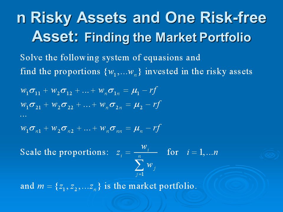
30. n Risky Assets and One Risk-free Asset: Finding the Market Portfolio

32. A Numeric Example Find the market portfolio if there are only two risky assets, A and B, and a risk-free asset rf. μ A =10%; μ B =5%; σ A =12%; σ B =6%; ρ AB =(-0.5) and rf=4%

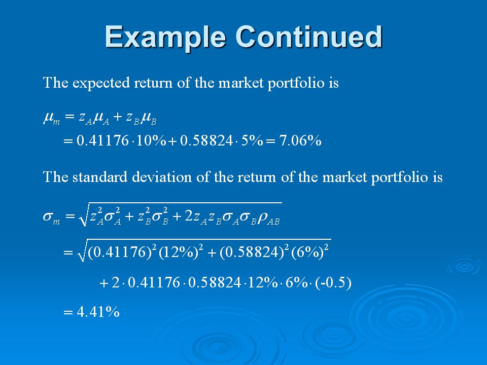
33. Example Continued

35. Practice Problems BKM Ch. 8: 1-7, 11-14 Mathematics of Portfolio Theory: Read and practice parts 11-13.