Download presentation
Presentation is loading. Please wait.

1
Productivity and Taxes as Drivers of FDI Heckman Selection model Rahul Anand Econ 764 class presentation

2
Outline Theoretical framework of the determinants of FDI flow Analytical framework with productivity as a driving force M&A FDI flows Greenfield FDI flows Extending the framework to include corporate taxation as an additional driving force Econometric Approach: Heckman Selection model Empirical Evidence

3
Theoretical Framework Focus on bilateral FDI flows among members of OECD Study of two set of driving forces- Productivity Taxation Important feature of this model: fixed set up costs of new investments (distinguishing FDI flows from portfolio flows)
")
4
Two margins of FDI decision- Intensive margin: determining the magnitude of flows, based on standard marginal productivity conditions Extensive margin: whether to make new investment at all Productivity and Taxes may affect the two margins in different, possibly conflicting ways Set up costs can be industry-specific, giving rise to two way rich-rich, as well as rich-poor, FDI flows

5
A Stripped-Down Model of Foreign Direct Investment Source to host FDI flows typically include many observations with zero flows, may be an indication of existence of fixed set up costs A stripped down model of FDI with fixed set up costs

6
Model Consider a pair of source and host country Free capital mobility, fixing world interest rate at r Host country: denoted by H Source country : denoted by S A representative industry whose product serves for both consumption and investment Firms last for two periods

7
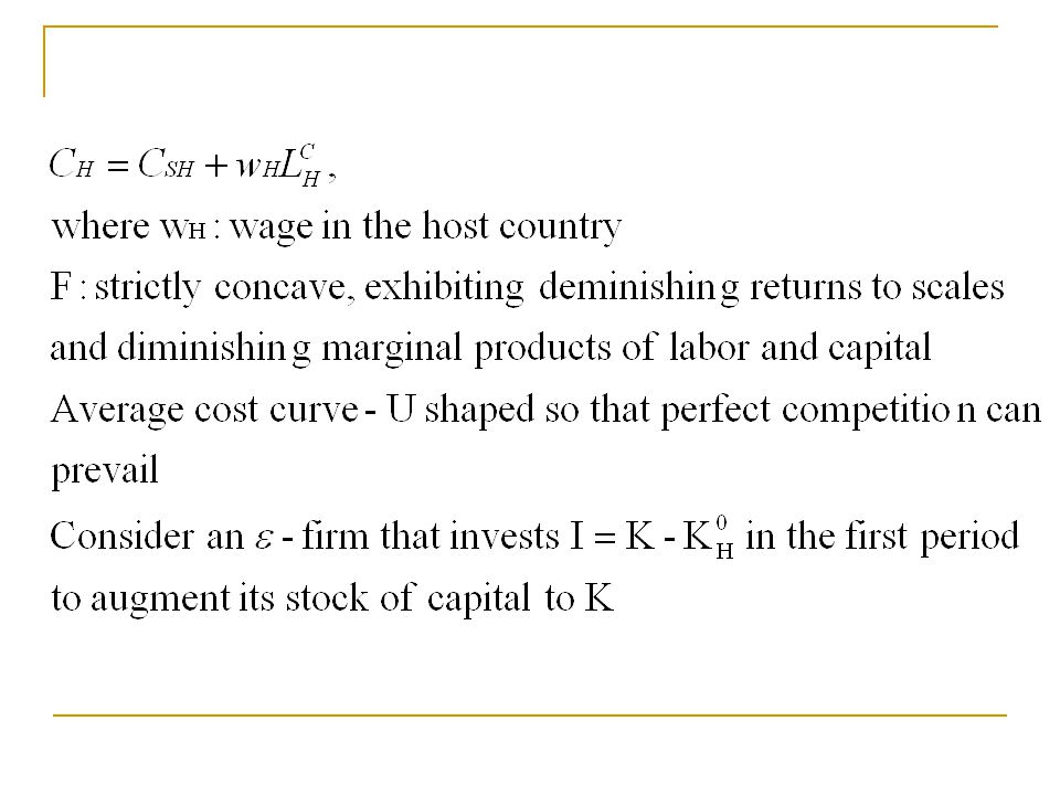
In 1 st period: continuum of N H firms that differ by an idiosyncratic productivity factor, ε Firm with productivity factor of ε is referred to as ε –firm G(.): Cumulative distribution of ε g(.) : Density function Number of ε-firms = N H *g(ε) K H 0 = initial net capital stock of each firm (assumed same for all firms) If invest I, augmented capital stock K = K H 0 +I
: Cumulative distribution of ε g(.) : Density function Number of ε-firms = N H *g(ε) K H 0 = initial net capital stock of each firm (assumed same for all firms) If invest I, augmented capital stock K = K H 0 +I")
8
Gross output in period 2: A H F(K,L)(1+ε) A H = country (H) specific aggregate productivity parameter Assume, C H = fixed set up cost of investment (same for all firms, independent of ε) Fixed cost has two components- C SH = cost borne by FDI investor in his own country (management time and other expenses at home headquarters) Cost incurred in host country: assume it involves labor input only, L H C
(1+ε) A H = country (H) specific aggregate productivity parameter Assume, C H = fixed set up cost of investment (same for all firms, independent of ε) Fixed cost has two components- C SH = cost borne by FDI investor in his own country (management time and other expenses at home headquarters) Cost incurred in host country: assume it involves labor input only, L H C")
13
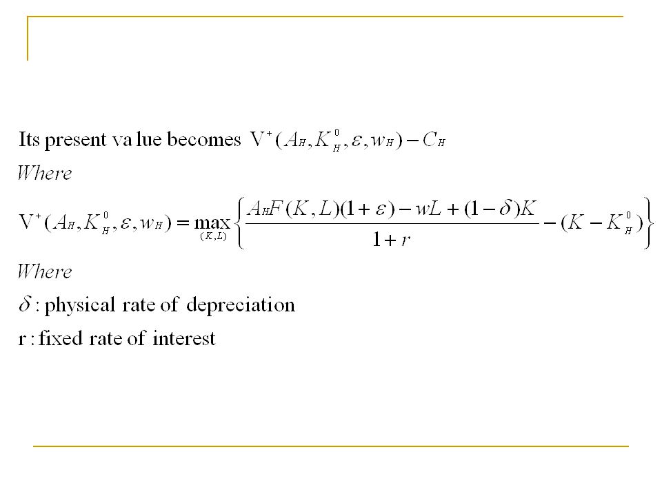
Firm invests if PV(Investment)>PV(without investment) A firm with higher ε (higher productivity firm) benefits more from investment
>PV(without investment) A firm with higher ε (higher productivity firm) benefits more from investment")
14
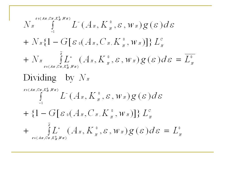
Therefore a cutoff ε exists(ε 0 ) such that an ε– investment firm will make a new investment if and only if ε >ε 0 V + (A H,K H O, ε 0,w H ) –C H = V - (A H,K H O, ε 0,w H ) w H is determined in equilibrium by a clearance in the labor market
 such that an ε– investment firm will make a new investment if and only if ε >ε 0 V + (A H,K H O, ε 0,w H ) –C H = V - (A H,K H O, ε 0,w H ) w H is determined in equilibrium by a clearance in the labor market")
16
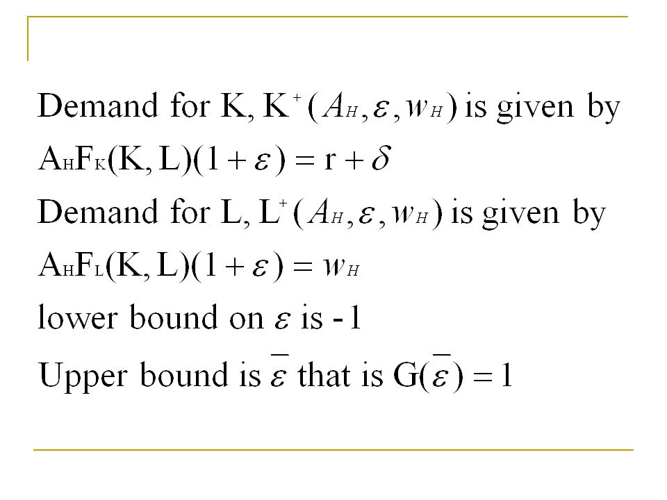
Labor abundance is manifested in wage differences If labor per firm in host > labor per firm in source (i.e, L H o > L S o ) In addition no. of firms –a measure of abundance of entrepreneurship- abundance of labor means scarcity of entrepreneurship If wages equal then demand per firm is same in both countries and market clearing condition could not hold for both countries Hence, w H < w S (Host employ more worker per firm, in equilibrium Source firm effectively more productive)
.")
17
Mergers and Acquisitions FDI M & A: acquisitions of existing host firms Source country entrepreneurs endowed with some intangible capital, or know how, stemming from their specialization/expertise comparative advantage: Set up cost by source FDI investors in host country < Set up cost by host investors in host country C H *= C SH * + w H L H C < C H

18
Foreign investor can bid up the direct investors of the host country in the purchase of the investing firm in the host country Each firm (with ε >ε 0 ) is purchased at its market value, V + (A H,K H O, ε 0,w H ) –C H New owner also invests: K + (A H,ε,w H ) –K H O in the firm
 is purchased at its market value, V + (A H,K H O, ε 0,w H ) –C H New owner also invests: K + (A H,ε,w H ) –K H O in the firm")
19
The amount of FD Investment made by a firm with ε >ε 0

20
Aggregate Productivity Shock: Flow and Selection How shock to A H affects FDI flows to the host country? Case 1: w H Fixed Three positive effects of positive shock on the notiaonal FDI on Flow equation Raises the marginal productivity of capital, increasing the amount of investment made by each investing firm It raises the value of each such firms, increasing the acquisition price which is a part of notional FDI Increasing the number of firms purchased by FDI investors (by lowering ε 0 )
.")
21
Derivation of results:

22
Selection Condition Equation: A rise in A H reduces the likelihood that ε 0 exceeds ε¯ (as profitability of investment increases, the threshold condition for investment decreases) So the likelihood of satisfying the selection condition increases implying the realization of notional FDI flow Thus a positive aggregate productivity shock raises actual FDI through both the flow and selection condition equation
 So the likelihood of satisfying the selection condition increases implying the realization of notional FDI flow Thus a positive aggregate productivity shock raises actual FDI through both the flow and selection condition equation")
23
Case 2: w H not fixed Wage is determined through market clearing conditions Increase in demand of labor raises w H, raising the fixed set up cost w H L H C COUNTERING THE ABOVE THREE EFFECTS With unique equilibrium the initial effects are likely to dominate these subsequent counter effects, so the notional FDI still rises (governed by the flow equation)
")
24
Effect on Selection Condition Equation Increase in set up cost reduces the advantage of carrying out positive FDI flows at all As w H rises ε 0 rises, reducing the likelihood of satisfying the selection condition So, the follow up effects of a positive shock works in the opposite direction and may dominate it A S has no effect : as free capital mobility

25
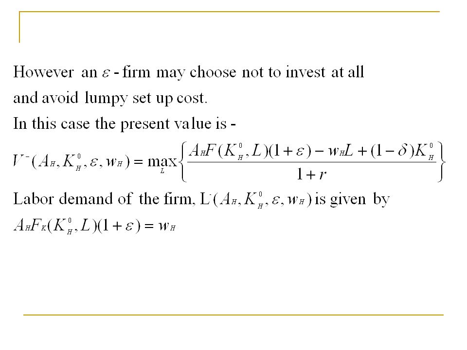
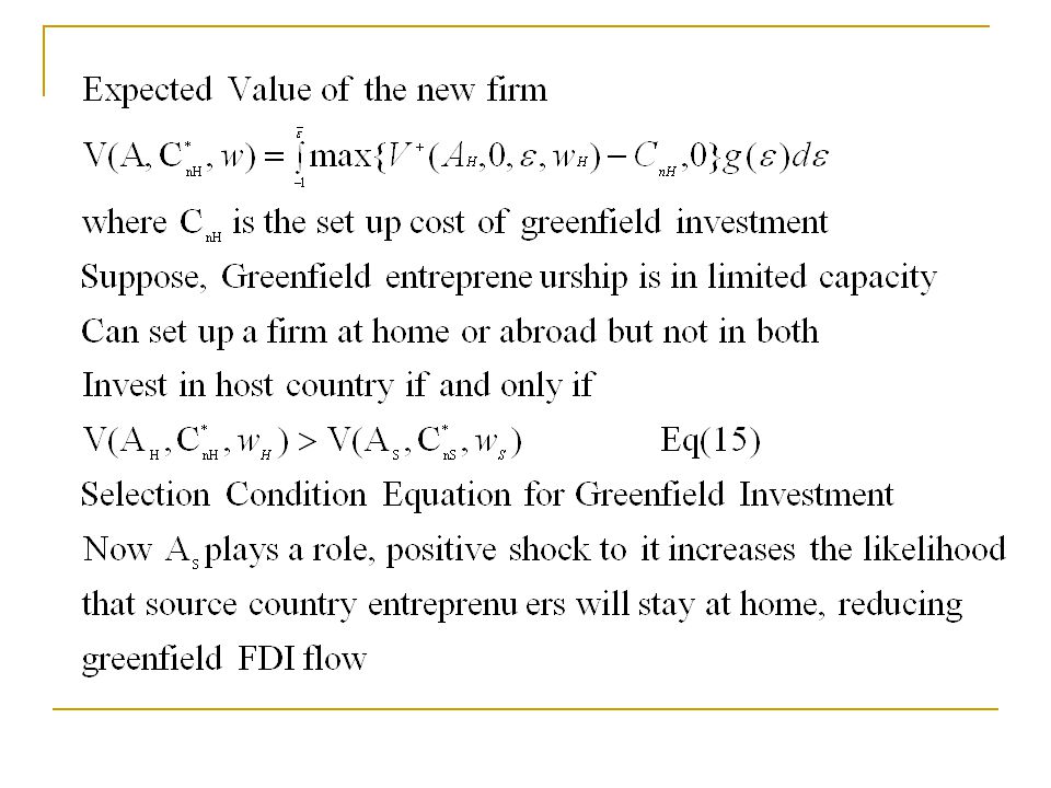
Greenfield FDI Establishing a new firm (where K H O =0) Newcomer doesn’t know in advance ε of the potential firm and takes G(.) as the CDF. Assumption- ε is revealed before he decides whether or not to make new investment

27
Entrepreneur must decide which host country to invest in and should also outbid competitors from other source countries

28
Effect of Positive Productivity Shocks Positive Shock to A H Positive effects on both the notional FDI flows and on the likelihood of these flows to actually materialize Positive Shock to A S Doesn’t affect the notional flows but reduces the likelihood of such flows to occur at all Positive Shock to A H ’(productivity of other potential hosts) Likelihood of having greenfield FDI is negatively affected
 Likelihood of having greenfield FDI is negatively affected")
29
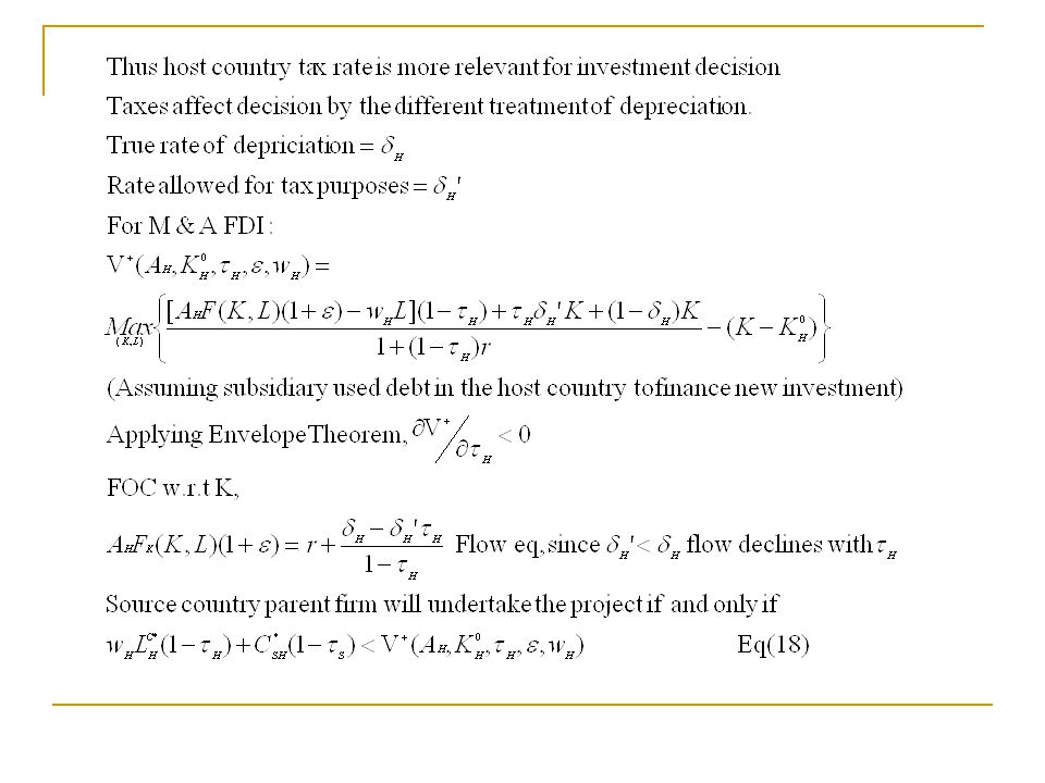
Source Country and Host Country Corporate Taxation Tax rates of the source country and host country may have different effect on the two decisions (flow and selection condition equations) Case of a parent firm developing a new product line Develop it at home and produce it at a subsidiary abroad Determined by productivities and tax considerations
 Case of a parent firm developing a new product line Develop it at home and produce it at a subsidiary abroad Determined by productivities and tax considerations")
30
Issue of Double Taxation Income of a foreign affiliate typically taxed by the host country If source country also taxes: double taxation Double taxation is typically relieved at the source country level (by granting exemption or granting tax credits) In practice, foreign source income is far from being taxed at the source country rate Various reduced rates for foreign source income Taxed only upon repatriation
 In practice, foreign source income is far from being taxed at the source country rate Various reduced rates for foreign source income Taxed only upon repatriation")
32
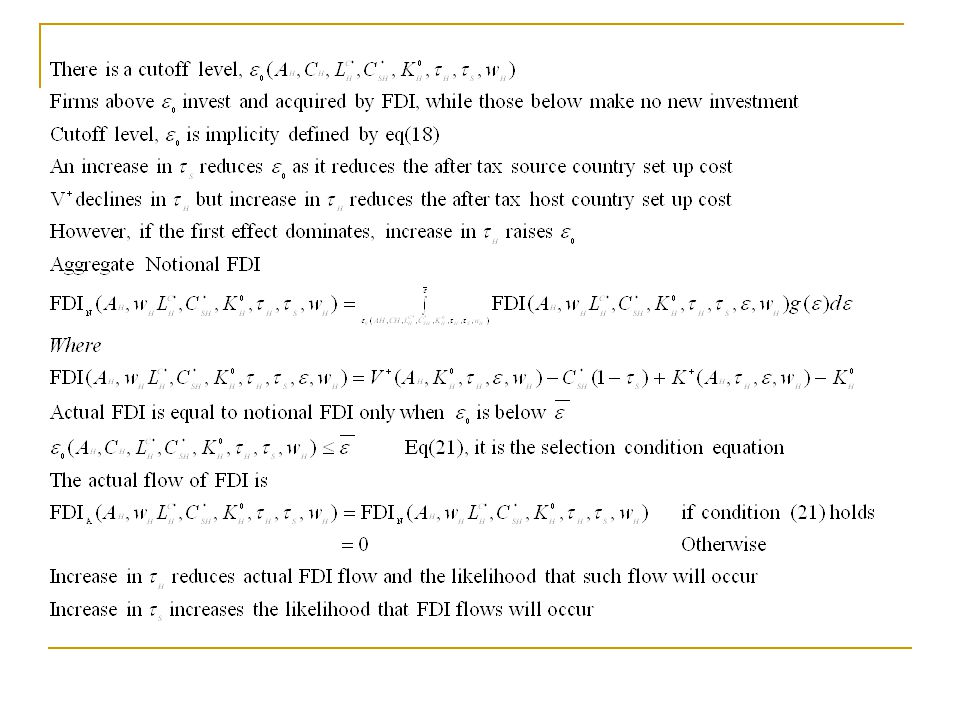
Effect of tax rates Tax rate in source country ς s affects positively the decision by a parent firm to invest in host ς H has a negative effect on this decision ς s is irrelevant for the determination of the magnitude of FDI flows which are negatively affected by ς H

34
Econometric Approach FDI flow two fold decisions: Whether to invest: “threshold” selection eq. How much to invest: “flow/gravity” eq. There may be zero actual flows Hence, selection of actual (s,h) countries endogenous (as opposed to exogenous in traditional gravity models) So, Heckman Selection Model used
 countries endogenous (as opposed to exogenous in traditional gravity models) So, Heckman Selection Model used.")
35
Heckman Selection Model Jointly estimate the likelihood of surpassing the threshold and the magnitude of the FDI flow (provided threshold is surpassed)
")
36
Flow Equation

37
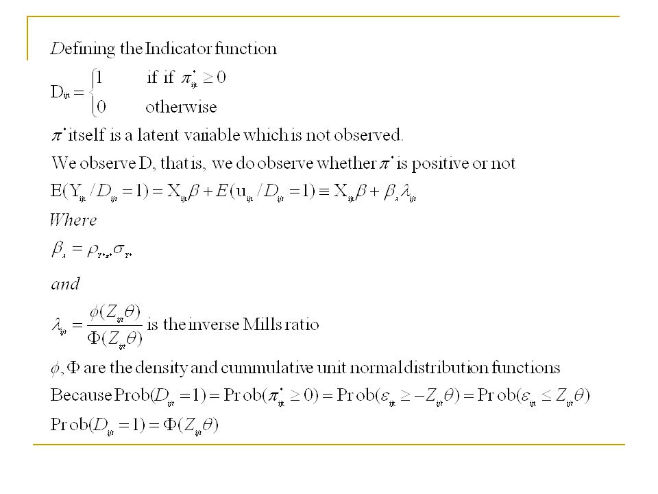
Y* ijt can be positive or negative Y ijt is zero not only when Y* ijt is negative but also when Y* ijt is positive but below the threshold profit π* ijt = π*’ ijt / σ π*’ = (W ijt ρ– C ijt ) / σ π*’ π*’ ijt : indicates if FDI will be made or not (depending on positive or negative) W ijt : explanatory variables C ijt : fixed cost of setting up new investment ρ : vector of coefficients σ π*’ : standard deviation of π*’
 / σ π*’ π*’ ijt : indicates if FDI will be made or not (depending on positive or negative) W ijt : explanatory variables C ijt : fixed cost of setting up new investment ρ : vector of coefficients σ π*’ : standard deviation of π*’")
38
Set up cost C* ijt = A ijt δ + v ijt A ijt : explanatory variables δ : vector of coefficients v ijt : error term Substituting for C* ijt in the previous equation

39
π* ijt = Z ijt θ + ε ijt Where, Z ijt = (W ijt, A ijt ) θ = (ρ/σ π*’,- δ/σ π*’ ) ε ijt = - v ijt /σ π*’
 θ = (ρ/σ π*’,- δ/σ π*’ ) ε ijt = - v ijt /σ π*’")
40
Assuming and u ijt and v ijt are normally distributed with zero means. It follows that ε ijt is N(0,1). The error terms ε ijt and u ijt are bivariate normal:
. The error terms ε ijt and u ijt are bivariate normal:.")
42
Maximum Likelihood method is employed to estimate the flow coefficient vector β and the selection coefficient vector θ λ ijt depends on X ijt. So from equation 7.8. OLS estimates of β confined to positive observations of Yijt is biased because such estimates include also the effect of X ijt on Y ijt through the term β λ λ ijt

43
TT’ M M’ A’ B’ A B XLXL XHXH X ijt Y ijt Y*=β X X Y=b X OLS X R S

44
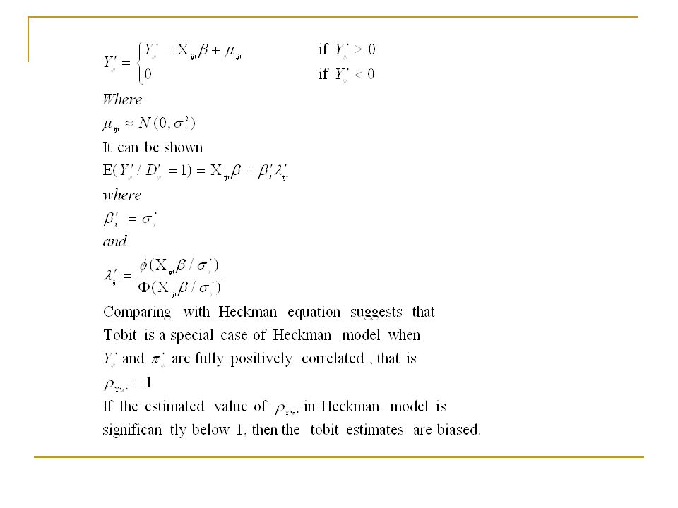
The Tobit Model Actual FDI flow may be zero even when notional FDI flows are not. A significant portion of a typical sample is zero, but is roughly continuously distributed for positive values. In such cases Tobit model is often employed.

46
Empirical Analysis Productivity and Tax Rate as Determinants of FDI flows

47
Data and Descriptive Statistics Standard Mass Variables Source and host population sizes Distance Variables Physical distance Whether two countries share a common language Economic Variables Source and host GDP per capita Difference in years of schooling Financial risk rating

48
Control for country and time fixed effects Dependent Variable in all flow equations: Log of FDI flow The main variables are grouped as follows: Standard Country Characteristics Real GDP per capita Source and host GDP per capita Difference in years of schooling Financial risk rating

49
Source and Host Characteristics Physical distance Whether two countries share a common language Productivity Corporate tax rates Productivity Approximated by output per worker- measured by purchasing power parity-adjusted real GDP per worker At times instrumented by capital to labor ratio and years of schooling

50
Corporate Tax Rates Statutory rates or by the effective average rates compiled by Devereux, Griffith, and Klemm At times instrumented by the statutory corporate tax rates and GDP per capita No smoothing of data done: to investigate the effects of the explanatory variables over the business cycle Data on FDI flows from International Direct Investment (IDI): bilateral flows among 18 OECD countries during 1987-2003 Deflated by US CPI (Urban Consumers)
: bilateral flows among 18 OECD countries during Deflated by US CPI (Urban Consumers)")
51
Empirical Evidence Since labor productivity and FDI flows both affected by other variables not controlled for (such as business cycle variables, interest rate and unemployment rate), alternatives in results presented First regression: only labor productivity Second regression: labor productivity is instrumented by the capital-to-labor ratio, years of schooling and country fixed effects
, alternatives in results presented First regression: only labor productivity Second regression: labor productivity is instrumented by the capital-to-labor ratio, years of schooling and country fixed effects")
52
Tax Variables First, statutory tax rates Another alternative is the effective tax rates compiled by Devereux, Griffith, and Klemm (difference between the cost of capital in the corporate sector and the tax-free interest) Also use the statutory corporate tax rates, GDP per capita, and country fixed effects as instruments to generate the fitted values for the effective tax rates
 Also use the statutory corporate tax rates, GDP per capita, and country fixed effects as instruments to generate the fitted values for the effective tax rates")
53
Predicted Effects M&AGreenfield FlowSelectionFlowSelection Productivity increase, fixed wages Host++++ Source000- Productivity increase, flexible wages Host Source +Amb++ Tax Increase Host-- Source0+

54
Results Table A-2: Instrumented productivity and tax equation Coefficients on capital-to-labor, years of schooling are significant and positive Statutory tax rate and GDP per capita are positive and significant

55
Productivity as a Driver Table 4: column 1-uninstrument productivities, column 2- instrumented productivities Source GDP per capita has a positive and significant effect on flow equations in both columns Host GDP per capita has a positive and significant effect on flow equation in column 2 only Neither significant in selection equation

56
Existence of previous FDI (a dummy) may be indicative of low setup costs. Used as an exclusion restrictions in the selection equation. It is significant and positive Column 1 of Table 4 Productivity host: positive in both flow and selection but significant in only flow Productivity source: negative and significant in selection Both results consistent with the analytical framework

57
Column 2, Table 4: Productivity host: not significant Productivity source: negative and significant in flow and selection Results consistent with the model Figure 2 and Figure 3

58
Tax Variables First 3 columns of Table 5: 1 st column – statutory tax rate 2 nd column – effective tax rates 3 rd column – fitted effective tax rates Host tax rate – negative and significant effect on flow of FDI in flow equations Source tax rate - positive and significant effect on flow of FDI in flow equations Source tax has a positive and significant effect on the selection mechanism (as predicted by theory) but only in column 1 (it intensifies in column 4, with larger set of countries).
 but only in column 1 (it intensifies in column 4, with larger set of countries).")
59
Figure 4 and 5 When both set of drivers are used, a problem of multicolinearity arises. Estimates shown in A-3. Results don’t change in sign but there statistical significance weakens.

60
Conclusion Examined the role of productivity and corporate taxation as driving forces Important feature – fixed set up costs FDI flows: M&A Greenfield Differ in that alternate investment opportunities in host countries do not affect M&A

61
Effect of productivity shock on M&A considered. Under fixed wages it has three positive effects on notional flow of FDI Raises the marginal productivity of capital, increasing the amount of investment made by each investing firm It raises the value of each such firms, increasing the acquisition price which is a part of notional FDI Increasing the number of firms purchased by FDI investors (by lowering ε 0 ) Selection Equation Shock increases profitability hence notional FDI is realized
 Selection Equation Shock increases profitability hence notional FDI is realized.")
62
When wage rate flexible The three effects are countered by raising wage in the host country In selection condition the rising host country component of set up cost reduce the likelihood of positive FDI flows to occur. Source country shocks does not affect M&A Greenfield FDI Positive shock has positive effect on notional flows and likelihood of flow Positive source country shock reduces the likelihood of FDI flows

63
Empirical findings support the claims of the model Host output per worker has a positive effect in both the flow and selection equation, but significant only in flow equation Source country output per worker has a negative and significant effect on the selection mechanism Results are robust

64
Tax as driver Host tax rate has negative and significant effect on flow of FDI in flow equation Source tax rate has positive and significant effect in flow equation Magnitude increasing (source country tax has a depressing effect on their investment abroad) Results fairly robust Source tax – positive and significant effect on the selection mechanism
 Results fairly robust Source tax – positive and significant effect on the selection mechanism")
65
Effects intensifies for larger set of countries Simulations suggest marked differences in the sensitivity of flows from the US to OECD countries Sensitivity to flow in UK is positive and higher than EU and Japan. The sensitivity of these flows to taxes in UK is negative and high relative to other countries

66
Empirical Analysis Existence of Fixed Costs

67
Data and Variables OECD Countries (from OECD reports) 24 countries 1981-1998 FDI export from 17 OECD source countries to 24 OECD countries Three year average (to smooth the variables): six periods
 24 countries FDI export from 17 OECD source countries to 24 OECD countries Three year average (to smooth the variables): six periods")
68
Explanatory Variables Country Characteristics GDP or GDP per capita Population size Educational attainment (average years of schooling) Language Financial sound rating (inverse of financial risk rating) Source-Host Characteristics Geographical distance Common language (zero-one variable) Flows of goods Bilateral telephone traffic per capita (proxy for international distance)
 Language Financial sound rating (inverse of financial risk rating) Source-Host Characteristics Geographical distance Common language (zero-one variable) Flows of goods Bilateral telephone traffic per capita (proxy for international distance)")
69
Estimation GDP per capita : good predictor of direction of the direction of flows Frequency of flows Close to one among rich countries Very low or close to zero among poorer countries Source-Host differences in GDP per capita are not correlated with the volume of FDI flows (among the subset of country pairs with positive flows) Japan got 1.26% of its GDP from US, whereas Spain received 6.54% of its GDP from US
 Japan got 1.26% of its GDP from US, whereas Spain received 6.54% of its GDP from US")
70
Estimation of the Determinants of bilateral FDI flows Standard Mass Variables Source and host population sizes Distance Variables Physical distance Whether two countries share a common language Economic Variables Source and host GDP per capita Difference in years of schooling Financial risk rating

71
Control for country and time fixed effects Dependent Variable in all flow equations: Log of FDI flow deflated by the unit value of manufactured goods exports

72
Econometric Procedure Adopted 1. As a benchmark, ignoring the selection equation and estimating the gravity equation twice By treating all FDI flows in (s,h) pairs with no recorded FDI flows as “zeros” (OLS-zero) By excluding country pairs with no FDI flows (OLS-D) Assign a negligible value as a common low value for the value of the FDI flows for the zero-flow (s,h) pairs Here the lowest observed flow between any (s,h) country pair in the sample is chosen
 pairs with no recorded FDI flows as zeros (OLS-zero) By excluding country pairs with no FDI flows (OLS-D) Assign a negligible value as a common low value for the value of the FDI flows for the zero-flow (s,h) pairs Here the lowest observed flow between any (s,h) country pair in the sample is chosen.")
73
Rationale of including “zeros” in OLS-zero case: Observed zero flows could be because: Two countries don’t wish to have such flows even in the absence of fixed costs Set up costs are prohibitive Measurement error So under the assumption of no set up costs and measurement errors, (s,h) pairs with zero FDI flows truly indicate zero flows
 pairs with zero FDI flows truly indicate zero flows")
74
Tobit Assumptions No fixed costs All FDI flows that are below a certain low threshold level (“censor”) are due to measurement errors Tobit estimator Three “censor” levels considered Lowest 0.0 3.00
 are due to measurement errors Tobit estimator Three censor levels considered Lowest 0.0 3.00")
75
Heckman Selection Model To highlight the role of fixed setup costs against the two benchmarks Jointly estimate the maximum likelihood of the flow equation and the selection equation It accommodates both the measurement errors and a possible existence of setup costs

76
Binary Variable D ijt D i,j,t = 1 if country i exports positive FDI to country j at time t D i,j,t = 0, otherwise Assuming that the setup costs are lower if country i has invested in country j in the past D i,j,t-k could serve as an instrument in the selection equation (exclusion restriction)
")
77
Results All results confirm volume of FDI flows is not affected by deviations from long run averages of GDP per capita in the source and host countries Host country education level, relative to source-country counterpart: Tobit: significant effect on flow of FDI Heckman: manifests through selection and has no significant effect on the flow of FDI

78
Nonlinearity in FDI flows: parameters of interest in the OLS method estimated for different range of FDI flows OLS-zero has different coefficients from those of OLS-D regression Common language dummy: positive and significant Distance: negative and significant in all formulations

79
Host country financial sound rating: Significant (and positive) in only Heckman flow equation and OLS-D case Source country financial sound rating Significant and negative effect on FDI in the tobit cases and one of the two OLS cases (OLS-zero) Heckman method suggests that it works through the selection process rather than having a direct effect on FDI flows
 in only Heckman flow equation and OLS-D case Source country financial sound rating Significant and negative effect on FDI in the tobit cases and one of the two OLS cases (OLS-zero) Heckman method suggests that it works through the selection process rather than having a direct effect on FDI flows")
80
Existence of previous FDI flows: Significant and positive effect in the selection effect indicating that the existence of FDI flows in the past reduces the fixed cost of setting a new FDI Correlation between the error terms in the flow and the selection equations is negative and significant – additional evidence for the relevance of fixed set up costs

81
Few cases of negative flows in the sample, indicating liquidations of previous FDI A dummy variable for negative FDI flows as an instrument (reasonable as past FDI liquidations are correlated positively with past FDI flows, but not a priori correlated with current FDI flows) Tobit: positive role to this dummy for flows (Table 8.6) Heckman: positive effect comes through the selection mechanism
 Tobit: positive role to this dummy for flows (Table 8.6) Heckman: positive effect comes through the selection mechanism")
82
Evidence of Fixed Costs Significant correlation ρ between the error terms in the flow and selection equations indicates that the formation of an (s,h) pair of positive FDI, and the size of the FDI flows between this pair of countries are not independent process ρ negative is consistent with the setup cost hypothesis
 pair of positive FDI, and the size of the FDI flows between this pair of countries are not independent process ρ negative is consistent with the setup cost hypothesis")
83
Conclusion Some evidence of fixed costs In such case the OLS and Tobit estimates of the determinants of FDI flows is biased Heckman method suggests some of the determinants of FDI flows in OLS and Tobit in fact influence FDI through selection mechanism rather than directly through the flows of FDI

84
Thanks

Similar presentations