1. ACCURACY ASSESSMENT OF EARTH GRAVITY FIELD MODELS BY MEANS OF INDEPENDENT SATELLITE CROSSOVER ALTIMETRY J. Klokočník, J. Kostelecký, C.A. Wagner Presented at CEDR Workshop, Třešť, October 2004

2. Two basic types of tests

4. Radial error, historical data

5. Radial error, historical data, contribution by individual satellites

8. Theory (1)

12. Theory (2)

13. Method

14. How it works? Our method enriches the spectrum of methods of accuracy tests of the Earth gravity field models. We make use of independent single satellite crossover (SSC) residuals and latitude lumped coefficients (LLC). We are able to test lower degree and order harmonic geopotential coefficients of the gravity models. We correct SSC for all available corrections, we convert them to latitude lumped coefficient (LLC) discrepancies (see STEP 1) by a least squares adjustment (with some constraints on land area without altimetry data). We compute the LLC errors for the given orbit with testing altimetry data from the given (usually tentatively scaled or already calibrated) variance-covariance matrix of the harmonic coefficients of the tested model (STEP 2). Finally, we compare results of STEP 1 and STEP 2 in a statistic way; we compute RMS of power of LLC discrepancies and errors for the given orbit and covariance matrix for various orders over all latitudes with crossover data. This comparison confirms the tentative scale factor or leads to suggest its change.

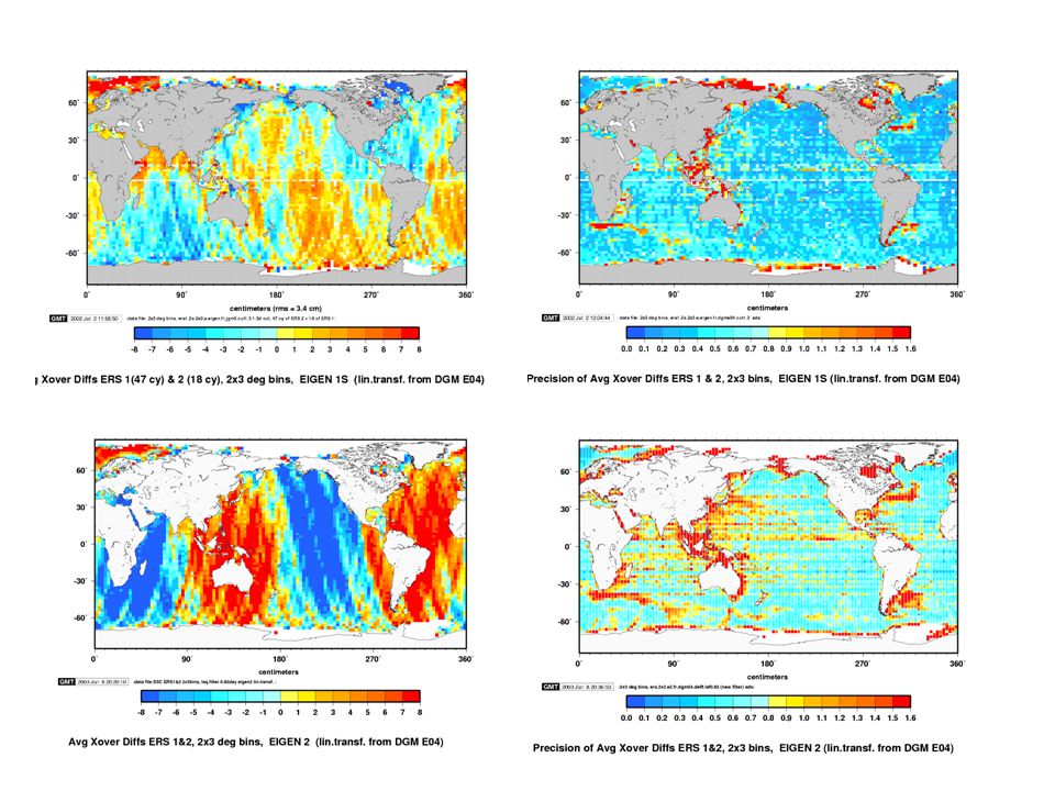
15. Test of linear transfer The processing steps from precision orbit determination to sea surface heights and SSC residuals is complex and time consuming. Thus the crossover residuals can be predicted (transformed) from one to another gravity model just by changing the relevant harmonic geopotencial coefficients. We call this procedure „linear transfer“. This is not a correct way but we performed various tests of the reliability to demonstrate that it is a good approximation to a „real world“. In the past we have available only gravity models mutually similar, like JGM 2 and JGM3. Here we work with the transfer from DGM E04 to GRIM5C1. Shown are RMS of power of LLC discrep.& errors for ERS 1/2 with GRIM5C1 calibrated covariance matrix, with GRIM5C1 linearly transferred (Pathfinder data) SSC and LLC, and with true GRIM5C1-based SSC (R. Scharroo). The SSC data is from the tandem mission interval. Clearly shown is a good agreement between the GRIM5C1 linearly transferred and true SSC/LLC, confirming again the transfer as a safety procedure, for our purpose.

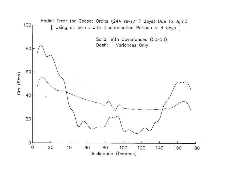
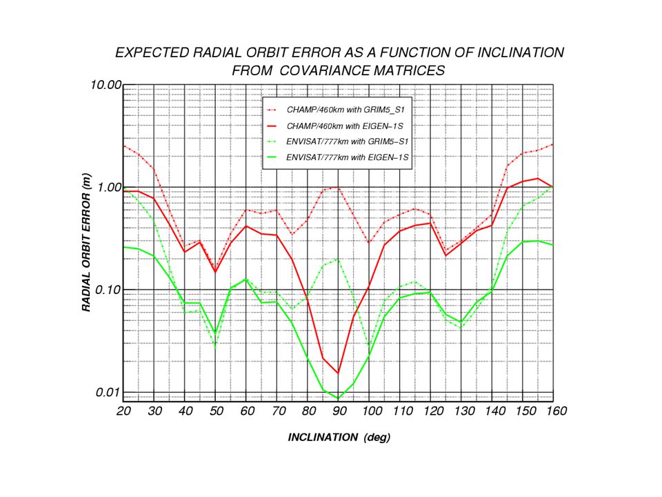
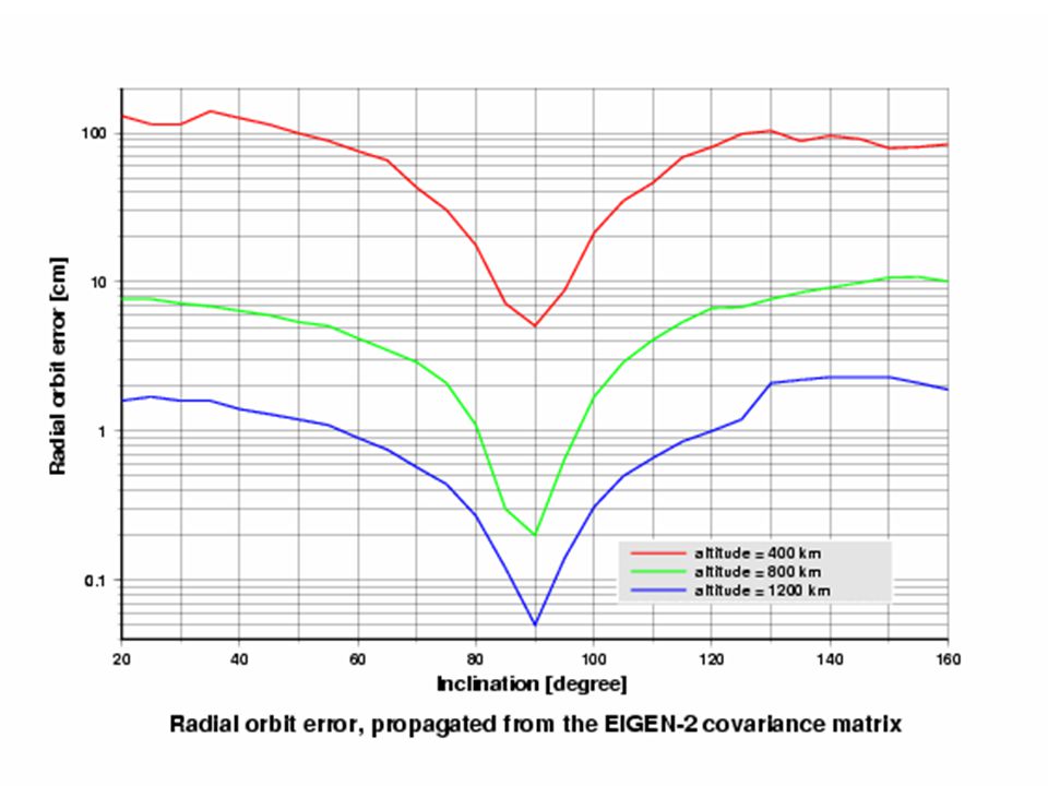
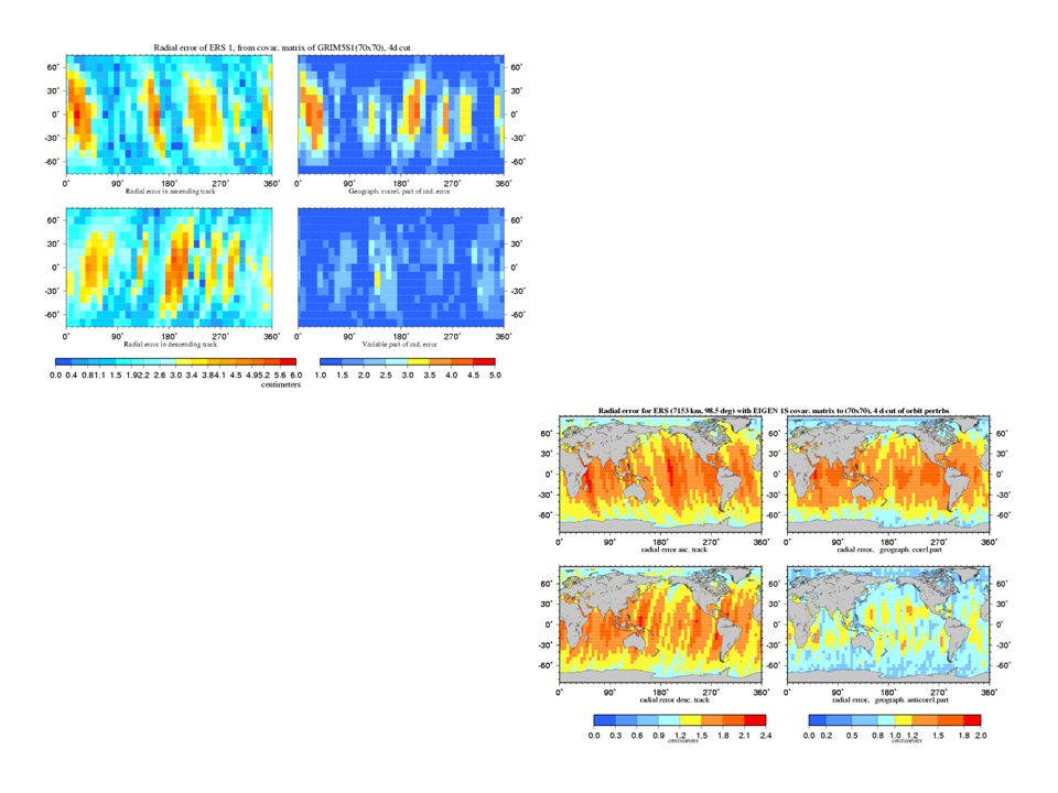
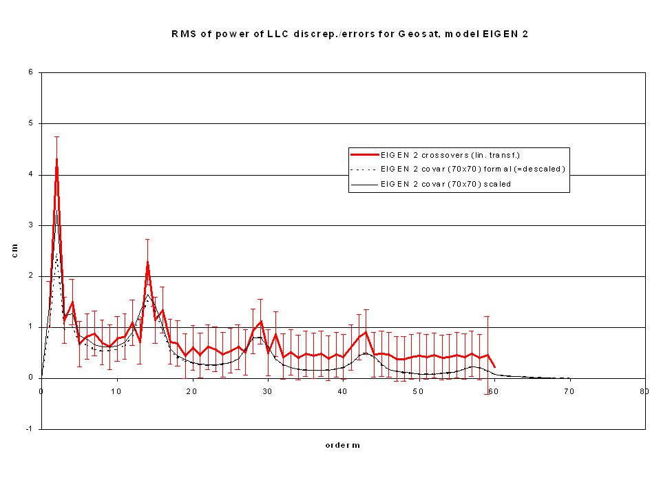
17. Is satellite altimetry precise enough to test newest gravity models with extensive sets of the CHAMP data? Three plots show the radial accuracy for various gravity models and selected orbits. Orbit improvement with the CHAMP data is remarkable - from about 1 meter with GRIM5S1 to several centimeters with EIGEN 1S and 2 in the radial direction for orbit of CHAMP, assuming the covariance matrix of EIGENs is well calibrated; the question is whether the altimetry still can test objectively such comprehensive solutions? The radial error decreased often but not always also for other orbits with inclinations and semimajor axes different from those of CHAMP. For ERS orbit type, SSC error was about 4 cm with GRIM5S1 and is about 3 cm with EIGEN 1S, for Geosat 11/8 cm respectively. Let us consider a signal to noise (s/n) ratio, where s means the SSC errors from covariance projections and n means SSC data errors. Due to long- term averaging of SSC (sometimes several years), we keep n below 1 cm; now for the best ERS1/2 and Geosat data available in 2003, it is often about 0.6/0.9 cm. Thus, s/n was and still is high enough to have our test statistically significant.

19. RMS of power of LLCdiscrep./errors and formal sd for ERS 1 and 2, model EIGEN1S -0.5 0 0.5 1 1.5 2 01020304050607080 order m cm EIGEN1S covar (70 x 70) EIGEN1S crossovers (CAW binned 2x3 deg) sd - sd + EIGEN1S crossovers (Pathfinder for tandem mission)

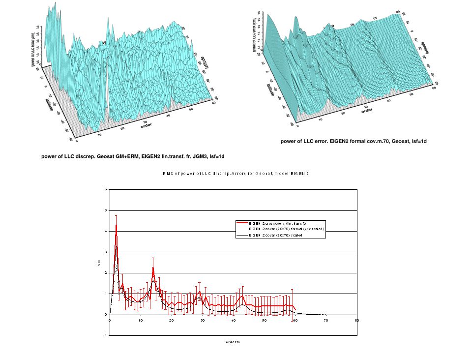
22. RMS of powers of LLC discrep./errors for Geosat, model EIGEN1S 0 1 2 3 4 5 6 7 01020304050607080 order m cm EIGEN1S crossovers (CAW) EIGEN1S covar (70 x 70) descaled EIGEN1S covar (70 x 70)

24. Summary (1) Goal: to test existing tentative or to suggest a new calibration factor for the formal covariance matrix of C_lm, S_lm of a gravity field model under evaluation Method: independent satellite crossover altimetry data and latitude lumped coefficients (LLC) are prerequisities for one of many methods to assess accuracy of the Earth gravity field models. LLC are linear combinations of harmonic geopotential coefficients over degrees, here restricted to the low and medium degree and order part of a gravity model (to degree about 50)

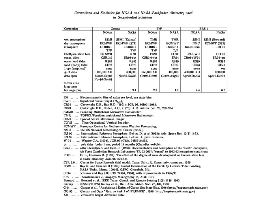
25. Summary (2) DATA: Long-term (multi-year), precise, month-to-month averaged single satellite crossover (SSC) seaheight differences over majority of world’s oceans (with preference to southern hemisphere) from ERS 1 and 2 (and partly Geosat), carefully corrected for a bunch of environmental (non-gravitational) effects, are used PROCEDURE: LLC discrepancies are derived from those SSC residuals LLC errors are computed by error propagation from tentatively scaled variance-covariance matrix of the tested model Powers of both LLC discrepancies and errors are compared

26. Summary (3) Models tested: GEM T2, JGM 2, 3, EGM 96, PGM 2000A, TEG 4, GRIM 5S1, GRIM 5C1, POEM G0, GS0.1, and EIGEN 1S. LLC errors presented for various orbits (CHAMP, ERS 1, 2, /ENVISAT, TOPEX/Poseidon/JASON, GFZ 1, Geosat/GFO) with scaled (or calibrated) covariances for JGM 3, EGM 96, PGM 2000A, GRIM5S1, C1, POEM GS0.1 and EIGEN 1S.

27. Conclusion (1) Accuracy assessment presented for JGM 3, EGM 96, PGM 2000A, GRIM5S1, C1 and EIGEN 1S (+test of internal consistency for TEG 4) with the following conclusions: GRIM 5 models have the calibrating factor 5 and our test confirms it as a fair choice. PGM 2000A is on the same accuracy level (for the part tested by SSCs) as was EGM 96 (PGM 2000A includes global circulation model POCM_4B). T/P orbit looks worse in PGM2000A than in EGM96. TEG 4 covariance matrix (provided by CSR for testing purposes) is sufficiently calibrated. TEG 4 looks very accurate for ERS-type orbits.

28. Conclusion (2) EIGEN 1S, whose covariance matrix is tentatively calibrated by degree dependent factor (45/2 for l=0, 45/l for 0 36), looks well calibrated in general, but might need to increase that scaling factor slightly, by about 30-50%. CHAMP data leads to a substantial improvement of the radial orbit error for satellites at inclination I=87 deg and in its vicinity; for T/P, EIGEN 1S provides in this test procedure worse result than GRIM 5S1 (which is part of EIGEN 1S).

29. ON THE FEASIBILITY OF ACCURACY ASSESSMENT OF UPCOMING GRAVITY FIELD MODELS BY MEANS OF ECGN ARRAY J. Kostelecký 2, J. Klokočník 1, P. Novák 2 1) CEDR, Astronomical Institute of the Czech Acad.of Science, CZ 2) CEDR, Research Institute of Geodesy, GO Pecný, CZ Presented at EUREF 2004, 2 - 5 June, Bratislava, Slovakia

30. Gravity field model is „nothing“ without reliable accuracy assessment of its geopotential coefficients and other quantities Testing the external accuracy of the Earth models becomes more an more important, with increasing accuracy of the models and decreasing access of TESTING data (sub)sets of the highest quality.

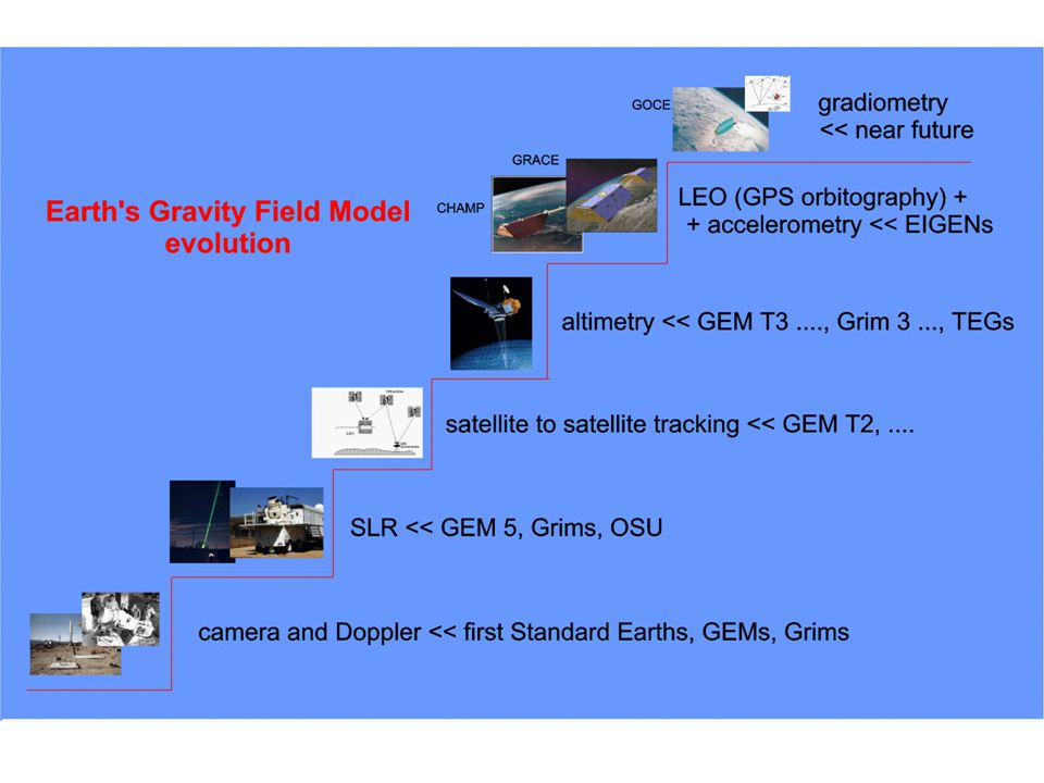
32. Evolution of the Earth gravity field models (EM) accuracy assessments - improving accuracy of EMs with time - new data – first used for testing EMs - then incorporated into the newest EMs of that time - higher and higher accuracy, resolution, reliability - large step in quality by altimetry - large step expected from satellite gradiometry the basic question HOW TO TEST EM WHICH IS EXPECTED (DUE TO DATA USED) TO BE THE MOST ACCURATE OF ALL MODELS TILL NOW AVAILABLE WHEN NO TESTING DATA OF COMPARABLE OR HIGHER ACCURACY IS AVAILABLE ?

33. Status in Earth gravity models (EM) accuracy testing General requirement: data of accuracy equal or higher than is the accuracy of the tested EMs. Problem in a near future… · What data is used? independent orbits, gravity anomalies, satellite-to-satellite tracking, crossover altimetry data (see example), satellite gradiometry in a near future. Problem: the new data is quickly incorporated into EMs. dependent data-subsets (Lerch’s statistics) · What quantities are used? 1) power spectra, various statistics, orbit overlaps, … Problem: often not actual test of accuracy, but only a test of internal precision or of consistency 2) Even actual accuracy tests (orbit predictions …) suffer from limited sensitivity to various degrees and orders of C lm, S lm in EMs. Various data types = different spectral sensitivity… 3) Comparison of satellite dynamics data and “GPS-levelling” How is the perspective? Bad. A new data type (gradiometry) and/or very accurate terrestrial data is needed

34. How to continue to test the Earth gravity field models (EM) when better (more accurate and reliable) satellite data than those used to compute the models will not be available?? WE NEED TERRESTRIAL DATA 1. Can we compare global ”smothed” EMs based (also) on satellite data with the point measurements on the ground ? YES 2. What ground instruments can we use ? SG and AG superconducting gravimeters (SG) as pseudo-continuous data source and absolute gravimeters (AG) as sporadic, additional data source, to use the POINT values after all reductions, no smoothing/averaging (as was frequently used) with the gravity anomalies in the past 3. How the distribution of the ground stations should be? Are new stations needed? As regular as possible, present situation shown on Figure is not optimum, new stations are needed outside Europe

35. Superconducting Gravimeter Network Conception (BKG) © J. Neumeyer, GFZ

36. Superconducting Gravimeter (SG) Gravity resolution: 10 -11 m/s 2 Measurement range: from seconds to years with a linear transfer function Drift: ~ 3 µgal/year linear Absolute Gravimeter (AG) Gravity resolution: 10 -10 m/s 2 Accuracy of 1 day measurement: 10 -8 m/s 2 Measurement range: from one day to years Drift: ~ 0 µgal/year

37. Absolute gravimeter FG5 Superconducting gravimeter

38. CHAMP Superconducting Gravimeter Gravity resolution Space resolution / 2 Sph.harm. coeff.-- Time resolution Long term stability (drift) 300 µgal 1 µgal 500 km 5000 km l max = 40 l max = 4 1 month10 seconds no drift ~ 3 µgal / year (linear) Performance Time variations of the gravity field are already studied using CHAMP and GRACE data – monthly solutions © J. Neumeyer, GFZ 1ngal (10 -11 m/s 2 ) point measurement

39. © J. Neumeyer, GFZ

40. Upper graph: green = SG: Gravity variations including long periodic tidal waves STA, SSA and SA red = SG: Monthly mean of gravity variations Lower graph: blue = CHAMP: monthly global gravity field solution for Metsahovi with added long periodic tidal waves red = SG: Monthly mean of gravity variations (deformation potential part only) Comparison by using long periodic tidal waves © J. Neumeyer, GFZ

41. We do not need the variations of the gravity field but the absolute values with utmost accuracy Crucial problem

42. Elementary error estimate (1) Present EMs transformed to geoid: 1 m global, 0.2 – 0.3 m ocean EMs (CHAMP, GRACE, combinations) transformed to geoid: 0.2 – 0.3 m global

43. Elementary error estimate (2) Relation between gravity change dg and vertical undulation dN dg = - 0.3086 dN rms error of vertical (~geoid) undulation m dN = m dg /0.3086 Numerically m dg (SG + AG) = 5 μGal > m dN = 1.5 cm with error of hydrological corrections: m dN = 2.5 cm 20 – 30 cm versus 2 – 3 cm great potential of SG+AG for checking EMs

44. Method There is a possibility how to invert Stokes’s coefficients of geopotential into observed values of ground gravity. The model can be summarized as follows: 1- synthesize the geopotential coefficients on the surface of the reference sphere (geocentric sphere upon which a spherical harmonic expansion of the coefficients reduces to the Laplace harmonics); this step results in mean values of geopotential defined over a selected grid of spherical coordinates 2- invert the mean values of geopotential through an integral equation of Green’s kind into the gradient of geopotential at a particular point on the surface of the Earth; direct integration can be used due a band-limited character of geopotential 3- project this gradient into the direction of a local plumb line and compare it with an observed value of gravity.

45. List of problems to be solved (1) Spherical harmonic coefficients of geopotential derived from observables of various satellite missions provide a continuous representation of geopotential that is averaged both in time and space. For example, for the GRACE mission 30-day estimates of the coefficients up to degree 150 can be recovered that represent the geopotential function spatially averaged to some 100 km. This constitutes the major problem in comparing satellite- based estimates of geopotential with the ground reference. Namely a completely different spatial resolution must be dealt with while time averaging can also be applied to ground data. Possible solution: remove the high-frequency signal from ground reference (effect of close topographical masses).

46. List of problems to be solved (2) The spherical harmonic description also suggests that geopotential is a harmonic function in a certain domain. This condition results in a uniformly converging spherical harmonic series. Strictly speaking this condition is not satisfied for a general point inside the so-called Brilloiun sphere that may result in an unexpected effect of higher-degree terms in the expansion. It might be a good idea to expend the domain, where geopotential is harmonic, also for a region between the geoid and the Brilloiun sphere. Possible solution: remove the gravitational effect of global topography from satellite data and ground reference. In order to project the recovered potential gradient to the direction of the local plumb line, one should technically know its direction in some reference frame. In other words, one should know a deflection of verticals at the gravity station. The precise positioning of gravity stations is expected via GPS positioning. Possible solution: measuring astronomical coordinates.

47. Requirements on ECGN (1) Precise geocentric positions from space geodesy

48. Requirements on ECGN (2) Precise SG and AG measurements in dense and global network

49. Requirements on ECGN (3) Precise astronomical coordinates of a reference point of SG and AG instruments

50. Conclusions Point SG and AG data are potentially accurate enough to test the newest and future gravity field models (EM) based on satellite data (including altimetry and gradiometry). There is a possibility how to invert C lm, S lm from EMs to the point ground gravity values. We are aware of various problems connected with such accuracy tests and we have here presented a list of the problems to be solved. Better distribution of SG data, new SG and AG stations - ECGN sites - are needed and some of the SG/AG gravity reduction models must be improved.