Download presentation
Presentation is loading. Please wait.

1
GEOG 425/525 GPS Concepts and Techniques
John Benhart, Ph.D. Indiana University of PA Dept. of Geography & Regional Planning

2
What Are Global Positioning Systems (GPS)?
")
3
What is GPS Used For?

4
The Historical Context of the Global Positioning System (GPS)
The origins of surveying: Efforts to measure distance on the earth’s surface Efforts to specify location on the earth’s surface Efforts to determine property/land boundaries How?

5
How Eratosthenes Estimated the Earth’s Size

6
Early Estimates of the the Earth’s Size

7
1753 French Survey Establishes that the Earth Bulges at the Equator

8
The Basics of Surveying
Definition: The science of measuring and mapping relative positions above, on, or below the surface of the earth; or establishing such positions from a technical plan or title description Types: Plane surveying: Does not take into account the curvature of the earth Geodetic surveying: measurements covering larger distances where the curvature of the earth must be taken into account

9
Surveying: History Evidence of surveying has been recorded as early as 5,000 years ago Ancient Egyptian surveyors called harpedonapata (“rope stretcher” Ropes and knots were tied at pre-determined intervals to measure distances The triangle (later formalized by Pythgoras) was discovered to derive a right angle easily by using a rope knotted at 3,4, and 5 units Early Egyptian levels that were essentially plumb lines were derived
 was discovered to derive a right angle easily by using a rope knotted at 3,4, and 5 units. Early Egyptian levels that were essentially plumb lines were derived.")
10
Surveying: History Surveying inventions
Lodestone used to identify magnetic north Thomas Diggs invents an instrument used to measure angles called the theodolite in the mid-1500s Jean Praetorius invents the plane table in 1610 W.J. Young invents the transit based on the theodolite, which “flips” to allow back sighting in 1831

11
Theodolite

12
How a Theodolite Works

13
Plane Table and Alidade

14
Surveyor’s Transit

15
Total Station

16
The Basics of Surveying
Starting from a position with a known location and elevation, known as a “benchmark,” the distance and angles to the unknown point are measured Using a leveled theodolite or total station Distance: previously chains, now lasers Horizontal angle: from compass on theodolite Vertical Angle: sighted in on a measuring or leveling rod at the location in question

19
The Historical Context of the Global Positioning System (GPS)
1978 – launch of first GPS satellite 1982 – macrometer prototype tested at MIT 1984 – geodetic network densification in Montgomery, Co. PA 1989 – Launch of first Block II satellite; Wide Area GPS concept tested 1990 – GEOID90 for NAD83 datum established 1993 – Real-time kinematic GPS implemented 1996 – First US GPS policy expressed in presidential directive 1999 – US GPS modernization initiative 2000 – Selective availability (SA) deactivated
 deactivated.")
20
Overview of GPS - Logic A continuous coverage of satellites exists within view of virtually every location on the earth’s surface (NAVSTAR) These satellites launch signals at recorded times on specific frequencies that can be “received” by units on the earth’s surface By calculating the amount of time it takes the signals from 4 satellites to reach a receiver on the earth surface, it is possible to determine the distance between the receiver and any satellite (pseudoranges) By using the intersection of the radii from 4 satellites, it is possible to determine exactly where a GPS receiver is located on the earth’s surface (trilateration) ** A huge amount of science and technology has to be applied for any of these conditions above to exist…
 By using the intersection of the radii from 4 satellites, it is possible to determine exactly where a GPS receiver is located on the earth’s surface (trilateration) ** A huge amount of science and technology has to be applied for any of these conditions above to exist…")
21
Overview of GPS - Objectives
The GPS was “conceived as a ranging system from known positions in space to unknown positions on land, at sea, in air and space.” (p.11) The original objectives of GPS were “instantaneous determination of position and velocity (i.e. navigation), and the precise coordination of time (i.e. time transfer).” “The global NAVSTAR Global Positioning System (GPS) is an all-weather space-based navigation system under development by the DoD to satisfy the requirements of the military forces to accurately determine their position, velocity and time in a common reference system, anywhere on or near Earth on a continuous basis.”
 The original objectives of GPS were instantaneous determination of position and velocity (i.e. navigation), and the precise coordination of time (i.e. time transfer). The global NAVSTAR Global Positioning System (GPS) is an all-weather space-based navigation system under development by the DoD to satisfy the requirements of the military forces to accurately determine their position, velocity and time in a common reference system, anywhere on or near Earth on a continuous basis.")
22
Overview of GPS GPS can be conceptually be divided into 3 segments:
Space Segment: the constellation of satellites Control Segment: tracking and monitoring of the satellites User Segment: varying user applications and receiver types

23
Overview of GPS Space Segment
The NAVSTAR constellation: 24 evenly-spaced satellites in 12-hour orbits inclined 55 degrees to the equatorial plane…each is assigned a pseudorandom noise code # (PRN code) Types: Block I, Block II, Block IIA, IIR, IIF, and Block III Continuous signal coverage of every location on the earth’s surface Satellite signals: launched at extremely-precisely recorded times (atomic clocks), and travel at the speed of light (through earth atmosphere) to receivers on the earth’s surface L1: MHz, L2: MHz
 Types: Block I, Block II, Block IIA, IIR, IIF, and Block III. Continuous signal coverage of every location on the earth’s surface. Satellite signals: launched at extremely-precisely recorded times (atomic clocks), and travel at the speed of light (through earth atmosphere) to receivers on the earth’s surface. L1: MHz, L2: MHz.")
26
Overview of GPS Control Segment
Master control station: located at the Consolidated Space Operations Center at Shriver Air Force Base, Colorado Springs, CO Collects monitoring data from global stations Calculates satellite orbits and clock parameters for each satellite…passed to ground control stations Responsibility for satellite control

27
Overview of GPS Control Segment
Monitoring Stations: Five located at Colorado Springs, Hawaii, Ascension Island (South Atlantic), Diego Garcia (Indian Ocean), Kwajalein (North Pacific) Precise atomic time standard Continuous calculation of satellite pseudoranges Official network for determining broadcast ephemerides Ground Control Stations Also located at Ascension, Diego Garcia, and Kwajalein Communication links to upload ephemeris, and clock information to NAVSTAR satellites
, Diego Garcia (Indian Ocean), Kwajalein (North Pacific) Precise atomic time standard. Continuous calculation of satellite pseudoranges. Official network for determining broadcast ephemerides. Ground Control Stations. Also located at Ascension, Diego Garcia, and Kwajalein. Communication links to upload ephemeris, and clock information to NAVSTAR satellites.")
28
GPS Monitoring Locations

29
Overview of GPS User Segment Military Users Civilian Users
Original envisioned users; have access to precise P-code satellite signals Civilian Users Range from recreational to GIS and survey grade applications – all made possible by federal infrastructure Receiver Types C/A code pseudorange; C/A code carrier phase; P-code carrier phase; Y-code carrier phase

30
GPS Summary The system is predicated on:
A constantly monitored constellation of satellites Very accurate time measurement The ability to determine satellite location The use of unique radio signals on specified wavelengths launched from satellites and received by receivers on the earth’s surface The ability to translate pseudoranges into recognized coordinates through trilateration

31
Reference Systems GPS satellites are orbiting earth and launching signals with time stamps…we are usually trying to determine locations on earth…to do this we have to define suitable coordinate and time systems 3 Types of reference systems that are relevant in the context of GPS Earth-fixed reference: the international terrestrial reference system Space-fixed reference: the international conventional celestial reference system Geodetic reference system

32
The Earth and Its Axis of Rotation
The Earth’s axis of rotation changes over time Why? 1) Mainly caused by the gravitational forces of the moon and the sun…as well as other celestial bodies 2) changes in the mass of earth-based phenomena Precession – a slight change in the direction of the axis of the rotating earth Nutation - a slight irregular motion in the axis of rotation of an axially symetrical body (planet) Polar Motion - the movement of the earth’s axis across its surface (~ 20 m westward since 1900)…due to motions in the earth’s core and mantle, and redistribution of water mass Who Cares? These factors cause the position of the earth in its orbit (revolution) around the sun to change over time (equinoxes and solstices)
 Mainly caused by the gravitational forces of the moon and the sun…as well as other celestial bodies 2) changes in the mass of earth-based phenomena. Precession – a slight change in the direction of the axis of the rotating earth. Nutation - a slight irregular motion in the axis of rotation of an axially symetrical body (planet) Polar Motion - the movement of the earth’s axis across its surface (~ 20 m westward since 1900)…due to motions in the earth’s core and mantle, and redistribution of water mass. Who Cares These factors cause the position of the earth in its orbit (revolution) around the sun to change over time (equinoxes and solstices)")
33
Precession Nutation Polar Motion

34
Precession: Cause The gravitational pull of the sun on the closest part of the oblate spheroid is stronger…

35
Precession: Result

36
Nutation

37
Reference Systems and Reference Frames
Reference Systems: the complete specification of a coordinate system, such as the origin, coordinate axes, coordinate units, etc. Reference Frames: consist of a set of identifiable points along with their coordinates, which serve as a realization of the reference system

38
International (Conventional) Celestial (Space) Reference System
The celestial reference system adopted by the International Astronomical Union (IAU) for high-precision positional astronomy Characteristics: Origin at the solar system barycenter (center of mass) and “space fixed” axis directions Has been chosen by the IAU as the “most appropriate coordinate system for expressing reference data on the positions and motions of celestial objects.”
 for high-precision positional astronomy. Characteristics: Origin at the solar system barycenter (center of mass) and space fixed axis directions. Has been chosen by the IAU as the most appropriate coordinate system for expressing reference data on the positions and motions of celestial objects.")
39
International (Conventional) Celestial (Space) Reference System
A set of specifications based on space-fixed axes defining the location of bodies in space For example, the base plane of the system is the extension of the earth’s equatorial plane at J (Jan. 1, 2000) Locations (of planets and stars) are specified based on declination (north-south) and right ascension (east)
 Locations (of planets and stars) are specified based on declination (north-south) and right ascension (east)")
41
Earth-Centered Earth-fixed Reference
The mass center of the earth is used as a reference Conventional Terrestrial Reference System: X axis is identical to the mean Prime (Greenwich) Meridian; Z axis is identical to the earth’s mean rotational axis (also called the Conventional International Origin (CIO)); Y axis points to the mean equatorial parallel See (the International Earth Rotation and Reference Systems Service)
 Meridian; Z axis is identical to the earth’s mean rotational axis (also called the Conventional International Origin (CIO)); Y axis points to the mean equatorial parallel. See (the International Earth Rotation and Reference Systems Service)")
42
International Union of Geodesy and Geophysics (1991) Resolution on the Conventional Terrestrial Reference System The International Union of Geodesy and Geophysics, Considering the need to define a Conventional Terrestrial Reference System (CTRS) which would be unambiguous at the millimeter level at the Earth's surface and that this level of accuracy must take account of relativity and of Earth deformation, and noting the resolutions on Reference Systems adopted by the XXIst General Assembly of the International Astronomical Union (IAU) at Buenos Aires, 1991, endorses the Reference System as defined by IAU at the XXIst General Assembly at Buenos Aires, 1991 and recommends the following definitions of the CTRS: 1) CTRS to be defined from a geocentric non-rotating system by a spatial rotation leading to a quasi-Cartesian system, 2) the geocentric non-rotating system to be identical to the Geocentric Reference System (GRS) as defined in the IAU resolutions, 3) the coordinate-time of the CTRS as well as the GRS to be the Geocentric Coordinate Time (TCG), 4) the origin of the system to be the geocenter of the Earth's masses including oceans and atmosphere, and, 5) the system to have no global residual rotation with respect to horizontal motions at the earth's surface.
 which would be unambiguous at the millimeter level at the Earth s surface and that this level of accuracy must take account of relativity and of Earth deformation, and. noting the resolutions on Reference Systems adopted by the XXIst General Assembly of the International Astronomical Union (IAU) at Buenos Aires, 1991, endorses the Reference System as defined by IAU at the XXIst General Assembly at Buenos Aires, 1991 and recommends the following definitions of the CTRS: 1) CTRS to be defined from a geocentric non-rotating system by a spatial rotation leading to a quasi-Cartesian system, 2) the geocentric non-rotating system to be identical to the Geocentric Reference System (GRS) as defined in the IAU resolutions, 3) the coordinate-time of the CTRS as well as the GRS to be the Geocentric Coordinate Time (TCG), 4) the origin of the system to be the geocenter of the Earth s masses including oceans and atmosphere, and, 5) the system to have no global residual rotation with respect to horizontal motions at the earth s surface.")
43
International (Conventional) Terrestrial (Earth) Reference System
 Terrestrial (Earth) Reference System")
45
The International Terrestrial Reference Frame
The Earth is constantly changing shape, because of plate tectonics and regional subsidence and/or used to represent the Earth when measuring its rotation in space. To be understood in context, when the motion of the Earth's crust is observed, it must be referenced. A Terrestrial Reference frame provides a set of coordinates of some points located on the Earth's surface. It can be used to measure plate tectonics, regional subsidence or loading and/or used to represent the Earth when measuring its rotation in space.

46
The International Terrestrial Reference Frame
This rotation is measured with respect to a frame tied to the celestial reference frame. The International Earth Rotation and Reference Systems Service (IERS) was created in 1988 to establish and maintain a Celestial Reference Frame, the ICRF, a Terrestrial Reference Frame, the ITRF. The Earth Orientation Parameters (EOPs) connect these two frames together. These frames provide a common reference to compare observations and results from different locations Reference locations are periodically evaluated for position change to re-define the reference frame The ITRF is regularly updated by the IERS…the latest frame is ITRF 2005
 was created in 1988 to establish and maintain a Celestial Reference Frame, the ICRF, a Terrestrial Reference Frame, the ITRF. The Earth Orientation Parameters (EOPs) connect these two frames together. These frames provide a common reference to compare observations and results from different locations. Reference locations are periodically evaluated for position change to re-define the reference frame. The ITRF is regularly updated by the IERS…the latest frame is ITRF")
50
Earth-Centered Earth-fixed Reference
World Geodetic System of 1984 (WGS84) The reference system utilized in GPS Provides the basic reference frame and geometric figure for the earth, based on the USDMA (Defense Mapping Agency’s) measurements and modeling of the earth from a geometric, geodetic, and gravitational standpoint, using techniques and technology available in 1984
 The reference system utilized in GPS. Provides the basic reference frame and geometric figure for the earth, based on the USDMA (Defense Mapping Agency’s) measurements and modeling of the earth from a geometric, geodetic, and gravitational standpoint, using techniques and technology available in")
51
Earth-Centered Earth-fixed Reference
World Geodetic System of 1984 WGS84: a = 6, m, f = 1/ Geocentric coordinate system originally realized from the coordinates of approx reference stations derived from TRANSIT observations Uniform specification of the earth’s size, shape, geoid surface characteristics, and reference station coordinates (unlike ITRF)
")
52
WGS84

55
Reference Systems Time – 3 major systems are used in GPS
Sidereal time: a measure of the earth’s rotation…defined as the hour angle of the vernal equinox (ie. Dynamical time: a uniformly-scaled time used to describe the motion of bodies in a gravitational field Terrestrial dynamic time may be used to describe satellite motion without taking into account the gravitational field of the sun Atomic time: time systems kept and defined by atomic clocks such as International Atomic Time (IAT) Uniformly-scaled time used in earth-centered coordinate systems Because of the slowing of the earth’s rotation with respect to the sun, “leap seconds” are used to create the Coordinated Universal Time System (UTC) In most cases UTC and GPS time are synonymous….it is the basis of GPS time calculations
 Uniformly-scaled time used in earth-centered coordinate systems. Because of the slowing of the earth’s rotation with respect to the sun, leap seconds are used to create the Coordinated Universal Time System (UTC) In most cases UTC and GPS time are synonymous….it is the basis of GPS time calculations.")
58
Reference Systems – Time Systems
GPS Calendar references Julian Date (JD): defines the number of mean solar days elapsed since January 1, 4713 BC Modified Julian Date (MJD): obtained by subtracting 2,400,000.5 days from JD Saves digits and has MJD start at midnight instead of noon GPS standard epoch (time, calendar): the atomic time scale implemented by the atomic clocks in GPS ground control stations and satellites GPS standard epoch was initiated on Jan. 6th, 1980 Current GPS reference to January 1, 2000 (J2000.0)
: defines the number of mean solar days elapsed since January 1, 4713 BC. Modified Julian Date (MJD): obtained by subtracting 2,400,000.5 days from JD. Saves digits and has MJD start at midnight instead of noon. GPS standard epoch (time, calendar): the atomic time scale implemented by the atomic clocks in GPS ground control stations and satellites. GPS standard epoch was initiated on Jan. 6th, Current GPS reference to January 1, 2000 (J2000.0)")
60
Inertial Frame of Reference
A reference frame in which… Newton’s first and second laws of motion are valid: inertia; acceleration Newton’s laws are valid in an environment that is nether rotating nor accelerating relative to other bodies By contrast, bodies may be subject to forces that result from the acceleration of the reference frame itself….

61
Earth-Fixed (Non-Inertial) Frame of Reference
One in which a body violates Newton’s law of Motion….that is, it is rotating or accelerating An example of an non-inertial frame is an earth-fixed coordinate reference, as the earth is rotating and body (satellite) motion is measured with respect to it
 motion is measured with respect to it.")
62
Inertial vs. Earth-fixed Reference
The inertial frame of reference is theoretical…. Therefore, a satellite’s orbit, and it relational location to the earth, must be translated into an earth-fixed reference One that takes into account the movement of the earth, including rotation, gravity impacts, etc.

63
Johannes Kepler – Scientist and Astronomer Developed important theories (laws) regarding planetary orbits…
 regarding planetary orbits… .")
65
Terms Relating to Keplerian Motion
Perigee: closest approach of a satellite with respect to the earth’s center of mass Apogee: most distant position (in an orbit) ” “ Nodes: intersections between the equatorial and orbital planes Anomaly: instantaneous position of a satellite within its orbit
 Nodes: intersections between the equatorial and orbital planes. Anomaly: instantaneous position of a satellite within its orbit.")
66
What are we Saying? The orbits of satellites around the earth can be described by an ellipse…that has the following characteristics (parameters): Right ascension of the ascending node Inclination of the orbital plane Argument of the perigree Semimajor axis of the orbital ellipse Numerical eccentricity of the ellipse Epoch of the perigree passage Orbits do not occur in an inertial environment

74
Keplerian Motion and Perturbed Motion
Perturbed motion is “characterized by the temporal variations of orbital parameters.” Caused by: gravitational forces (sun, moon), solar radiational pressure, eclipse periods, etc. Perturbed motion also causes the Keplerian orbit model specification to be modified
, solar radiational pressure, eclipse periods, etc. Perturbed motion also causes the Keplerian orbit model specification to be modified.")
76
Almanac A data file that contains the approximate orbit information of all satellites, which is transmitted by each satellite within its Navigation Message. It is transmitted by a GPS satellite to a GPS receiver, where it facilitates rapid satellite signal acquisition within GPS receivers.

77
Broadcast Ephemeris The "Broadcast Ephemeris (or Ephemerides)" for a satellite are the predictions of the current satellite position and velocity determined by the Master Control Station, uploaded by the Control Segment to the GPS satellites, and transmitted to the user receiver in the Data Message.
 for a satellite are the predictions of the current satellite position and velocity determined by the Master Control Station, uploaded by the Control Segment to the GPS satellites, and transmitted to the user receiver in the Data Message.")
80
Typical amount of Error (per Satellite)
Sources of Error Typical amount of Error (per Satellite) Beyond quality of equipment/size of antennea, etc. Satellite Atomic Clock Errors (corrected periodically) Satellite Orbit (Position) Errors Earth’s ionosphere (charged particles) Earth’s troposphere (moisture) Receiver Noise (local conditions, radio interference) Multipath Errors (bounce off buildings, etc.) Local Weather (moisture in air, lightning) Poor Satellite Geometry (GDOP) Receiver Clock Errors (corrected by 4th + Satellites) Satellite Atomic Clock Errors (corrected periodically) Satellite Orbit (Position) Errors Earth’s ionosphere (charged particles) Earth’s troposphere (moisture) Receiver Noise (local conditions, radio interference) Multipath Errors (bounce off buildings, etc.) Local Weather (moisture in air, lightning) Poor Satellite Geometry (GDOP) Receiver Clock Errors (corrected by 4th + Satellites) 1.5 m 2.5 m 5.0 m 0.5 m 0.3 m 0.6+ m
 Beyond quality of equipment/size of antennea, etc. Satellite Atomic Clock Errors. (corrected periodically) Satellite Orbit (Position) Errors. Earth’s ionosphere (charged particles) Earth’s troposphere (moisture) Receiver Noise (local conditions, radio interference) Multipath Errors (bounce off buildings, etc.) Local Weather (moisture in air, lightning) Poor Satellite Geometry (GDOP) Receiver Clock Errors (corrected by 4th + Satellites) Satellite Atomic Clock Errors. (corrected periodically) Satellite Orbit (Position) Errors. Earth’s ionosphere (charged particles) Earth’s troposphere (moisture) Receiver Noise (local conditions, radio interference) Multipath Errors (bounce off buildings, etc.) Local Weather (moisture in air, lightning) Poor Satellite Geometry (GDOP) Receiver Clock Errors (corrected by 4th + Satellites) 1.5 m. 2.5 m. 5.0 m. 0.5 m. 0.3 m m.")
81
GPS Masks: PDOP, Elevation, SNR
Allow the user to control the quality of the data accepted at the time of data collection (unacceptable readings are filtered out) PDOP Mask: Allows the recording of positions only when there is acceptable satellite geometry. Typically considers both quantity and quality of satellites (e.g., 4 satellites with good precision, or 6 with reasonable precision, or 8 with average precision) Elevation Mask: Sets minimum elevation above horizon for satellites to be used. The lower on the horizon a satellite is the more atmosphere the signal must pass through, thus the greater the potential for signal diffraction (inaccurate estimations of time/distance), as well as greater chance of multi-path errors. Also, with Differential Correction, insures that all satellites used are visible to base station as well as the field receiver. SNR (Signal to Noise Ratio) Mask: (higher is better, stronger signal) Filters out signals with excessive noise, using only those satellites with low noise (more accurate). SNR ranges from 0-35; 10-15 is typical, less than 5 is generally considered unusable.
 PDOP Mask: Allows the recording of positions only when there is. acceptable satellite geometry. Typically considers both quantity. and quality of satellites (e.g., 4 satellites with good precision, or. 6 with reasonable precision, or 8 with average precision) Elevation Mask: Sets minimum elevation above horizon for satellites to. be used. The lower on the horizon a satellite is the more. atmosphere the signal must pass through, thus the greater the. potential for signal diffraction (inaccurate estimations of. time/distance), as well as greater chance of multi-path errors. Also, with Differential Correction, insures that all satellites used. are visible to base station as well as the field receiver. SNR (Signal to Noise Ratio) Mask: (higher is better, stronger signal) Filters out signals with excessive noise, using only those. satellites with low noise (more accurate). SNR ranges from 0-35; is typical, less than 5 is generally considered unusable.")
82
Differential Correction
Can improve accuracy by up to 20 m. (50-90%) Requires local Base Station (w/in 100 miles) Requires “post-processing” (back in the lab) OR can be done on-the-fly using Real-Time DGPS Need better data – longer recording period, better GDOP More Base Stations near coasts (navigation) No effect on multi-path and/or receiver errors
 Requires local Base Station (w/in 100 miles) Requires post-processing (back in the lab) OR can be done on-the-fly using Real-Time DGPS. Need better data – longer recording period, better GDOP. More Base Stations near coasts (navigation) No effect on multi-path and/or receiver errors.")
85
Differential Correction
Compare GPS data file from Rover file (handheld unit) with a data file from a Base Station (at a known coordinate) for the exact same time period. Relies on the fact that receivers located relatively close together, will record similar errors from the same constellation of satellites. Uses the apparent “error” of the base station file to correct the corresponding error of the Rover file.
 with a data file from a Base Station (at a known coordinate) for the exact same time period. Relies on the fact that receivers located relatively close together, will record similar errors from the same constellation of satellites. Uses the apparent error of the base station file to correct the corresponding error of the Rover file.")
86
Differential Correction 2
10m Receiver (unknown Location) GPS Estimated Location Actual (Known) Position GPS Receiver Estimated Location Differentially Corrected Estimated Position Base Station (w/known coordinates) 10m
 GPS. Estimated Location. Actual (Known) Position. GPS Receiver. Estimated Location. Differentially Corrected Estimated Position. Base Station. (w/known coordinates) 10m.")
87
GPS Data Collection Procedure Using Trimble TerraSync
Once you start the unit up and check status (navigation screen) You will open a new data collection file .SSF file (default DDMMYYHH.SSF) A .DDF file is required data collection in an .SSF file (data dictionary) A default is provided if one is not selected The .DDF file becomes the template for the positional definition of features
 You will open a new data collection file. .SSF file (default DDMMYYHH.SSF) A .DDF file is required data collection in an .SSF file (data dictionary) A default is provided if one is not selected. The .DDF file becomes the template for the positional definition of features.")
88
THE GPS SIGNALS Each Satellite transmits two carrier waves L1 - frequency of MHz and a wavelength of approx 19cm L2 - frequency of MHz and a wavelength of approx 24cm The following satellite-specific signals, called the pseudo random noise (PRN) codes are modulated on the carrier waves: On L1: C/A (Coarse/Acquisition) code λ = approx 300m - Accessible to civilian users - Consists of a series of 1023 binary digits (called chips) that are unique to each satellite. - The chip pattern is repeated every millisecond P (precise) code λ = approx. 30m - Accessible only to military equipment On L2: P code only
 codes are modulated on the carrier waves: On L1: C/A (Coarse/Acquisition) code λ = approx 300m. - Accessible to civilian users. - Consists of a series of 1023 binary digits (called chips) that are unique to each satellite. - The chip pattern is repeated every millisecond. P (precise) code λ = approx. 30m. - Accessible only to military equipment. On L2: P code only.")
89
SVs transmit two microwave carrier (carry information) signals
L1 ( MHz): carries navigation message; SPS code (SPS: standard positioning service) L2 ( MHz): measures ionospheric delay 3 binary codes shift L1 and/or L2 carrier phases C/A code (coarse acquisition) modulates L1 carrier phase …repeating 1 MHz pseudo random noise (PRN) code …pseudo-random because repeats every 1023 bits or every millisecond…each SV has its own C/A code …basis for civilian SPS P-code (precise) modulates both L1 and L2 …long (7 days) pseudo random 10 MHz noise code …basis for PPS (precise positioning service) …AS (anti-spoofing) encrypts P-code into Y-code (need classified module for receiver) navigation message modulates L1-C/A; 50 Mhz signal ….describes satellite orbits, clock corrections, etc.
: carries navigation message; SPS code. (SPS: standard positioning service) L2 ( MHz): measures ionospheric delay. 3 binary codes shift L1 and/or L2 carrier phases. C/A code (coarse acquisition) modulates L1 carrier phase. …repeating 1 MHz pseudo random noise (PRN) code. …pseudo-random because repeats every 1023 bits or. every millisecond…each SV has its own C/A code. …basis for civilian SPS. P-code (precise) modulates both L1 and L2. …long (7 days) pseudo random 10 MHz noise code. …basis for PPS (precise positioning service) …AS (anti-spoofing) encrypts P-code into Y-code. (need classified module for receiver) navigation message modulates L1-C/A; 50 Mhz signal. ….describes satellite orbits, clock corrections, etc.")
91
GPS receiver produces replicas of C/A and/or P (Y) code
receiver produces C/A code sequence for specific SV

92
C/A code generator repeats same 1023 chip
PRN code sequence every millisecond PRN codes defined for 32 satellite ID numbers modern receivers usually store complete set of precomputed C/A code chips in memory

93
GPS Satellite Signals (Coarse Acquisition or C/A) Code Phase
Based on each satellite’s unique pseudo Random Noise Code (PRN) Each satellite’s PRN code is totally unique, and can be replicated by GPS receivers The receiver “slides” its code later and later in time until it matches up with the satellite’s code (code correlation) This is called “code phase lock”…however, even if this is achieved, there can be significant error Because the PRN codes are not that complicated (large cycle width ~ microsecond ~ 300 m. of error) Even with highly accurate code phase lock, error can be 5-10 meters (with the signal traveling at 180,000 miles per second)
 Each satellite’s PRN code is totally unique, and can be replicated by GPS receivers. The receiver slides its code later and later in time until it matches up with the satellite’s code (code correlation) This is called code phase lock …however, even if this is achieved, there can be significant error. Because the PRN codes are not that complicated (large cycle width ~ microsecond ~ 300 m. of error) Even with highly accurate code phase lock, error can be 5-10 meters (with the signal traveling at 180,000 miles per second)")
94
Code Signal Positioning
Subframe of message Receiver Signal Time Delay Matching Subframe Delayed Satellite Signal The ‘mis-match’ between the code patterns is a measure of the time the signal has taken to travel from satellite to receiver.

95
GPS Observables – Code Phase
The Pseudorange: The GPS receiver measures the distance between the satellite and antenna by measuring the time the signal takes to propagate from the satellite to the receiver…the pseudorange is the time offset multiplied by the speed of light

96
Code Pseudorange Based on travel time between when signal is sent and when it is received Time data also includes errors in both satellite and receiver clocks Δt = tr – ts = [tr(GPS)-δr] – [ts(GPS) – δs] Pseudorange given by R = c Δt = ρ + cΔδ Pseudo because of cΔδ (where Δδ = δs – δr) factor
-δr] – [ts(GPS) – δs] Pseudorange given by R = c Δt = ρ + cΔδ. Pseudo because of cΔδ (where Δδ = δs – δr) factor.")
97
Code Phase Acquisition
Code phase estimation PRN code characteristics Maximum autocorrelation at lag 0 Minimum auto-correlation in all other cases Minimum cross-correlation in all cases Generate local PRN code Perform circular correlation to obtain code phase Code phase is the circular shift of the local code that gives maximum correlation

98
receiver slides replica of code in time until
finds correlation with SV signal (codes are series of digital numbers)
")
99
if receiver applies different PRN code to SV signal
…no correlation when receiver uses same code as SV and codes begin to align …some signal power detected

100
when receiver and SV codes align completely
…full signal power detected usually a late version of code is compared with early version to insure that correlation peak is tracked

101
Acquisition Incoming code Generated code Correlation

102
Code tracking Enhance the accuracy of code phase obtained by acquisition Generate three local PRN codes 0.5 chips apart Early Prompt Late Correlate the local codes with incoming code Adjust code phase according to result of correlation
![]()
103
Code tracking Incoming code Early Prompt Late Correlation 1 0.5
Delay in chips -1 -0.5 0.5 1
![]()
104
GPS Satellite Signals Carrier Phase
The carrier signal has a much higher frequency than the PRN code, and therefore if “matched” has a much higher level of accuracy The carrier signal is ambiguous…that is it is much less differentiated than the PRN code The code correlation is used to “narrow down” the time frame of signal travel…then the carrier signal is used to very accurately determine signal travel time Used for high end mapping grade and survey grade GPS

105
Carrier Phase Based on the number of cycles (wavelengths) between satellite and receiver Phase data will include errors in both the satellite and receiver as well as an initial integer number, N

106
Combinations of Code and Carrier Phase
“Smoothing” of the code pseudorange using carrier phase correlation Several different algorithms

107
Carrier Phase Acquisition
Acquisition purpose Estimate coarse value of PRN code phase Estimate coarse value of carrier frequency Operates on 1ms blocks of data Corresponds to the length of a complete PRN code

108
Acquisition Carrier frequency estimation Generate local carrier
Adjust frequency until highest correlation is obtained

109
Acquisition Correlation

110
Acquisition Correct value for code phase and carrier frequency provides a peak correlation

111
Carrier Tracking Enhance the accuracy of the carrier frequency obtained by acquisition Generate local carrier signal Measure the phase error between incoming carrier and local carrier signal Adjust frequency until phase and frequency becomes stable Incoming signal NCO carrier generator Phase discriminator Loop filter PRN code
![]()
112
GPS signal Carrier wave Navigation data Carrier and data 1 data bit
1ms 20ms Carrier and data

113
GPS signal Carrier and data PRN code Resulting signal

114
GPS Navigation Message
The GPS navigation message consists of time-stamped data bits marking the time of transmission of each data bit frame A data (bit) frame is transmitted every 30 seconds and is comprised of 1500 bits, subdivided into bit subframes Subframe 1 – Clock correction (6 seconds) Subframes 2 and 3 – Ephemeris data for short segments of a satellite’s orbit Subframe 4 – Ionospheric corrections (GPS-UTC time offset) Subframe 5 – Almanac information An entire navigation message (25 data frames made up of 125 subframes) is sent over a 12.5 minute period
 frame is transmitted every 30 seconds and is comprised of 1500 bits, subdivided into bit subframes. Subframe 1 – Clock correction (6 seconds) Subframes 2 and 3 – Ephemeris data for short segments of a satellite’s orbit. Subframe 4 – Ionospheric corrections (GPS-UTC time offset) Subframe 5 – Almanac information. An entire navigation message (25 data frames made up of 125 subframes) is sent over a 12.5 minute period.")
115
GPS Navigation Message

117
Important tasks of a GPS receiver
Prepare received signals for signal processing Find satellites visible to the receiver For each satellite Find coarse values for C/A code phase and carrier frequency Find fine values for C/A code phase and carrier frequency Keep track of the C/A code phase and carrier frequency as they change over time Obtain navigation data bits Decode navigation data bits Calculate satellite position Calculate pseudorange Calculate position

118
Surveying with GPS Terminology
Code range: less complex, unambiguous signal…lower level of accuracy Carrier range: more complex, ambiguous signal…higher level of accuracy Real-time processing: position results must be available in the field immediately Post-processing: positional data are processed later

119
Surveying with GPS Terminology continued
Point positioning: a single receiver measures pseudoranges Differential positioning: an improved point positioning technique where corrections are applied to pseudoranges Relative positioning: two receivers are used, and simultaneously receive signals from the same satellites In general…point = navigation; relative = surveying, carrier phase; differential = code phase

120
Surveying with GPS Terminology continued
Static point positioning: derivation of point positions without correction; 10 m accuracy Static relative positioning (static surveying, carrier): most accurate; surveying technique; determination of the vector between two stationary receivers; cms. accuracy Kinematic relative positioning: two receivers perform observations simultaneously; one is stationary and one is moving
: most accurate; surveying technique; determination of the vector between two stationary receivers; cms. accuracy. Kinematic relative positioning: two receivers perform observations simultaneously; one is stationary and one is moving.")
121
Surveying with GPS – Observation Techniques
Point Positioning Standard Positioning Service is standard for civilian users Precise Positioning Service for military Differential GPS: Two or more receivers are used…one as a stationary “base”, and the other as a mobile “rover” Position correction; and pseudorange correction

122
Differential GPS Real-Time Post-Processing
Wide Area Augmentation System (WAAS) Originated for commercial air flights Post-Processing National Oceanic and Atmospheric Administration (NOAA) National Geodetic Survey (NGS) Continuously Operating Reference Station (CORS) network
 Originated for commercial air flights. Post-Processing. National Oceanic and Atmospheric Administration (NOAA) National Geodetic Survey (NGS) Continuously Operating Reference Station (CORS) network.")
123
Real-Time DGPS: The WAAS Network
Wide Area Augmentation System – Wide area ground reference stations (WRS) have been linked to form a U.S. WAAS network. Signals from GPS satellites are received by these precisely surveyed ground reference stations and any errors in the signals are identified. Each station in the network relays the data to one of two wide area master stations (WMS) where correction information for specific geographical areas is computed. A correction message is prepared and uplinked to a geostationary communications satellite (GEO) via a ground uplink station (GUS). This message is broadcast on the same frequency as GPS (L1, MHz) to GPS/WAAS receivers within the broadcast coverage area
 have been linked to form a U.S. WAAS network. Signals from GPS satellites are received by these precisely surveyed ground reference stations and any errors in the signals are identified. Each station in the network relays the data to one of two wide area master stations (WMS) where correction information for specific geographical areas is computed. A correction message is prepared and uplinked to a geostationary communications satellite (GEO) via a ground uplink station (GUS). This message is broadcast on the same frequency as GPS (L1, MHz) to GPS/WAAS receivers within the broadcast coverage area.")
124
Wide Area Augmentation System (WAAS)
")
125
Base Station Data: Where Does it Come From?
In many cases, base station data in the United States is obtained from the National Oceanic and Atmospheric Administration (NOAA) National Geodetic Survey (NGS) USNGS administers a program called CORS – Continuously Operating Reference Stations Data from a network of base stations across the US is available…including customized data sets
 National Geodetic Survey (NGS) USNGS administers a program called CORS – Continuously Operating Reference Stations. Data from a network of base stations across the US is available…including customized data sets.")
126
Surveying with GPS – Relative Positioning
“…the highest accuracies are achieved in the relative positioning mode with observed carrier phases.” Processing of baseline vectors Static relative positioning Kinematic relative positioning Pseudokinematic relative positioning

127
Surveying with GPS – Planning a GPS Survey
The Federal Geodetic Control Subcommittee (FGCS) has classified GPS surveys based on the levels of accuracy necessary A & B – very high accuracy geodetic control 1st, 2nd , 3rd – surveying, engineering, topographic mapping The higher the accuracy requirements, the more planning required
 has classified GPS surveys based on the levels of accuracy necessary. A & B – very high accuracy geodetic control. 1st, 2nd , 3rd – surveying, engineering, topographic mapping. The higher the accuracy requirements, the more planning required.")
128
Planning a GPS Survey GPS Survey Planning Parameters: Primitives
Site characteristics (obstructions, cover, etc.) Satellite configurations (number, constellation dispersion, data quality) Number and type of receivers Primitives Where, When, How Long, Quality
 Satellite configurations (number, constellation dispersion, data quality) Number and type of receivers. Primitives. Where, When, How Long, Quality.")
129
Planning a GPS Survey When – determination of the optimum daily observation period(s) The period when the maximum number of satellites can be observed simultaneously The period when the most advantageous constellation of SV azimuth/elevation combinations is “in view” Use of Plan modules available on receivers and/or lab software

130
What have We Covered Context of the GPS Structure of the GPS
Reference Systems Earth-fixed, Space-fixed, Geodetic Time systems Satellite orbits Specification and characteristics Keplerian motion; perturbed motion Characteristics of Trimble GeoXH and GeoXT GPS receivers GPS Satellite Signals Code phase; pseudoranges Carrier phase; ambiguity

131
What have We Covered Combination of Code and Carrier phases (smoothing) GPS Navigation message explanation Explanation of PathFinder Office and TerraSync softwares Hands-on use of PathFinder Office and TerraSync softwares Data Dictionary expanation/development Field Data Collection High Accuracy (survey-grade) GPS
 GPS.")
132
What You Should Have Obtained
Project experience Needs assessment Database design Data development Final Project documents (portfolio) References Other?
 References. Other")
133
TRANSFORMATION PARAMETERS AND THEIR RATES FROM ITRF94 TO OTHER FRAMES
SOLUTION T1 T2 T D R R R3 EPOCH Ref. cm cm cm " " " IERS Tech. Note #, page RATES T1 T2 T D R R R3 cm/y cm/y cm/y 10-8/y .001"/y .001"/y .001"/y ITRF RATES ITRF ITRF ITRF ITRF ITRF

134
X,Y,Z (Lat, Lon, h) based on the definition of WGS84 ellipsoid
 based on the definition of WGS84 ellipsoid")
135
World Geodetic System 1984 (WGS 84)
The original WGS 84 reference frame established in 1987 was realized through a set of Navy Navigation Satellite System (NNSS) or TRANSIT (Doppler) station coordinates Significant improvements in the realization of the WGS 84 reference frame have been achieved through the use of the NAVSTAR Global Positioning System (GPS). Currently WGS 84 is realized by the coordinates assigned to the GPS tracking stations used in the calculation of precise GPS orbits at NIMA (former DMA). NIMA currently utilizes the five globally dispersed Air Force operational GPS tracking stations augmented by seven tracking stations operated by NIMA. The coordinates of these tracking stations have been determined to an absolute accuracy of ±5 cm (1s).
 or TRANSIT (Doppler) station coordinates. Significant improvements in the realization of the WGS 84 reference frame have been achieved through the use of the NAVSTAR Global Positioning System (GPS). Currently WGS 84 is realized by the coordinates assigned to the GPS tracking stations used in the calculation of precise GPS orbits at NIMA (former DMA). NIMA currently utilizes the five globally dispersed Air Force operational GPS tracking stations augmented by seven tracking stations operated by NIMA. The coordinates of these tracking stations have been determined to an absolute accuracy of ±5 cm (1s).")
136
World Geodetic System 1984 (WGS 84)
Using GPS data from the Air Force and NIMA permanent GPS tracking stations along with data from a number of selected core stations from the International GPS Service for Geodynamics (IGS), NIMA estimated refined coordinates for the permanent Air Force and DMA stations. In this geodetic solution, a subset of selected IGS station coordinates was held fixed to their IERS Terrestrial Reference Frame (ITRF) coordinates.
, NIMA estimated refined coordinates for the permanent Air Force and DMA stations. In this geodetic solution, a subset of selected IGS station coordinates was held fixed to their IERS Terrestrial Reference Frame (ITRF) coordinates.")
137
World Geodetic System 1984 (WGS 84)
Within the past years, the coordinates for the NIMA GPS reference stations have been refined two times, once in 1994, and again in The two sets of self-consistent GPS-realized coordinates (Terrestrial Reference Frames) derived to date have been designated: WGS 84 (G730 or 1994) WGS 84 (G873 OR 1997) , where the ’G’ indicates these coordinates were obtained through GPS techniques and the number following the ’G’ indicates the GPS week number when these coordinates were implemented in the NIMA precise GPS ephemeris estimation process. These reference frame enhancements are negligible (less than 30 centimeters) in the context of mapping, charting and enroute navigation. Therefore, users should consider the WGS 84 reference frame unchanged for applications involving mapping, charting and enroute navigation.
 derived to date have been designated: WGS 84 (G730 or 1994) WGS 84 (G873 OR 1997) , where the ’G’ indicates these coordinates were obtained through GPS techniques and the number following the ’G’ indicates the GPS week number when these coordinates were implemented in the NIMA precise GPS ephemeris estimation process. These reference frame enhancements are negligible (less than 30 centimeters) in the context of mapping, charting and enroute navigation. Therefore, users should consider the WGS 84 reference frame unchanged for applications involving mapping, charting and enroute navigation.")
138
Differences between WGS 84 (G873) Coordinates and WGS 84 (G730), compared at 1994.0
Station Location NIMA Station Number D East (cm) D North (cm) D Ellipsoid Height (cm) Air Force Stations Colorado Springs Ascension Diego Garcia(<2 Mar 97) Kwajalein Hawaii NIMA Stations Australia Argentina England Bahrain Ecuador US Naval Observatory China *Coordinates are at the antenna electrical center.
 D North (cm) D Ellipsoid Height (cm) Air Force Stations. Colorado Springs Ascension Diego Garcia(<2 Mar 97) Kwajalein Hawaii NIMA Stations. Australia Argentina England Bahrain Ecuador US Naval Observatory China *Coordinates are at the antenna electrical center.")
139
World Geodetic System 1984 (WGS 84)
The WGS 84 (G730) reference frame was shown to be in agreement, after the adjustment of a best fitting 7-parameter transformation, with the ITRF92 at a level approaching 10 cm. While similar comparisons of WGS 84 (G873) and ITRF94 reveal systematic differences no larger than 2 cm (thus WGS 84 and ITRF94 (epoch ) practically coincide). In summary, the refinements which have been made to WGS 84 have reduced the uncertainty in the coordinates of the reference frame, the uncertainty of the gravitational model and the uncertainty of the geoid undulations. They have not changed WGS 84. As a result, the refinements are most important to the users requiring increased accuracies over capabilities provided by the previous editions of WGS 84.
 reference frame was shown to be in agreement, after the adjustment of a best fitting 7-parameter transformation, with the ITRF92 at a level approaching 10 cm. While similar comparisons of WGS 84 (G873) and ITRF94 reveal systematic differences no larger than 2 cm (thus WGS 84 and ITRF94 (epoch ) practically coincide). In summary, the refinements which have been made to WGS 84 have reduced the uncertainty in the coordinates of the reference frame, the uncertainty of the gravitational model and the uncertainty of the geoid undulations. They have not changed WGS 84. As a result, the refinements are most important to the users requiring increased accuracies over capabilities provided by the previous editions of WGS 84.")
140
World Geodetic System 1984 (WGS 84)
The global geocentric reference frame and collection of models known as the World Geodetic System 1984 (WGS 84) has evolved significantly since its creation in the mid-1980s primarily due to use of GPS. The WGS 84 continues to provide a single, common, accessible 3-dimensional coordinate system for geospatial data collected from a broad spectrum of sources. Some of this geospatial data exhibits a high degree of ’metric’ fidelity and requires a global reference frame which is free of any significant distortions or biases. For this reason, a series of improvements to WGS 84 were developed in the past several years which served to refine the original version.
 has evolved significantly since its creation in the mid-1980s primarily due to use of GPS. The WGS 84 continues to provide a single, common, accessible 3-dimensional coordinate system for geospatial data collected from a broad spectrum of sources. Some of this geospatial data exhibits a high degree of ’metric’ fidelity and requires a global reference frame which is free of any significant distortions or biases. For this reason, a series of improvements to WGS 84 were developed in the past several years which served to refine the original version.")
141
Other commonly used spatial reference systems
North American Datum 1983 (NAD83) State Plane Coordinate System (SPCS) based on NAD83 Universal Transverse Mercator (UTM)
 State Plane Coordinate System (SPCS) based on NAD83. Universal Transverse Mercator (UTM)")
142
North American Datum (NAD)
NAD27 established in 1927 defined by ellipsoid that best fit the North American continent, fixed at Meades Ranch in Kansas over the years errors and distortions reaching several meters were revealed In 1970’s and 1980’s NGS carried out massive readjustment of the horizontal datum, and redefined the ellipsoid The results is NAD83 (1986) based on earth-centered ellipsoid that best fits the globe and is more compatible with GPS surveying in 1990’s state-based networks readjustment and densification, accuracy improvement with GPS (HARN and CORS networks)
 based on earth-centered ellipsoid that best fits the globe and is more compatible with GPS surveying. in 1990’s state-based networks readjustment and densification, accuracy improvement with GPS (HARN and CORS networks)")
143
NAD 83 Defining Parameters
Parameter Notation Magnitude Semi-major Axis a meters Reciprocal of Flattening /f Datum point – none Longitude origin – Greenwich meridian Azimuth orientation – from north Best fitting – worldwide X,Y,Z (Lat, Lon, h) based on the definition of GRS80 ellipsoid
 based on the definition of GRS80 ellipsoid.")
144
State Plane Coordinate System
Based on Lambert and Transverse Mercator projections Developed in 1930’s and redefined in 1980’s and 90’s NAD ellipsoid was projected to the conical (Lambert) and cylindrical (Transverse Mercator) flat surfaces Allowed the entire USA to be mapped on a set of flat surfaces with no more than one foot distortion in every 10,000 feet (maximum scale distortion 1 in 10,000) Coordinates used are called easting and northing; derived from NAD latitude, longitude and ellipsoidal parameters
 and cylindrical (Transverse Mercator) flat surfaces. Allowed the entire USA to be mapped on a set of flat surfaces with no more than one foot distortion in every 10,000 feet (maximum scale distortion 1 in 10,000) Coordinates used are called easting and northing; derived from NAD latitude, longitude and ellipsoidal parameters.")
145
Lambert projection

146
Lambert projection

147
Transverse Mercator Projection

148
State Plane Coordinate System
The scale of the Lambert projection varies from north to south, thus, it is used in areas mostly extended in the east-west direction Conversely, the Transverse Mercator projection varies in scale in the east-west direction, making it most suitable for areas extending north and south Both projections retain the shape of the mapped surface Each state is usually covered by more than one zone, which have their own origins – thus, passing the zone boundary would cause the coordinate jump!

150
Universal Transverse Mercator, UTM
Developed by the Department of Defense for military purpose It is a global coordinate system Has 60 north-south zones numbered from west to east beginning at the 180th meridian The coordinate origin for each zone is at its central meridian and the equator

151
Universal Transverse Mercator
UTM zone numbers designate 6-degree longitudinal strips extending from 80 degrees south latitude to 84 degrees north latitude UTM zone characters designate 8-degree zones extending north and south from the equator There are special UTM zones between 0 degrees and 36 degrees longitude above 72 degrees latitude, and a special zone 32 between 56 degrees and 64 degrees north latitude

152
UTM Zones Each zone has a central meridia. Zone 14, for example, has a central meridial of 99 degrees west longitude. The zone extends from 96 to 102 degrees west longitude Easting are measured from the central meridian, with a 500 km false easting to insure positive coordinates Northing are measured from the equator, with a 10,000 km false northing for positions south of the equator

154
Ohio State Plane (Lambert projection, two zones) and UTM Coordinate Zone
 and UTM Coordinate Zone")
155
Universal Transverse Mercator, UTM

156
Vertical Datum Definition 1/2
Horizontal control networks provide positional information (latitude and longitude) with reference to a mathematical surface called sphere or spheroid (ellipsoid) By contrast, vertical control networks provide elevation with reference to a surface of constant gravitational potential, called geoid (approximately mean see level) this type of elevation information is called orthometric height (height above the geoid or mean sea level) determined by spirit leveling (including gravity measurements and reduction formulas). Height information referenced to the ellipsoidal surface is called ellipsoidal height. This kind of height information is provided by GPS
 with reference to a mathematical surface called sphere or spheroid (ellipsoid) By contrast, vertical control networks provide elevation with reference to a surface of constant gravitational potential, called geoid (approximately mean see level) this type of elevation information is called orthometric height (height above the geoid or mean sea level) determined by spirit leveling (including gravity measurements and reduction formulas). Height information referenced to the ellipsoidal surface is called ellipsoidal height. This kind of height information is provided by GPS.")
157
Height Systems Used in the USA
Orthometric Normal (orthometric normal) Dynamic Ellipsoidal Variety of height systems (datums) used requires careful definition of differences and transformation among the systems
 Dynamic. Ellipsoidal. Variety of height systems (datums) used requires careful definition of differences and transformation among the systems.")
158
Vertical Datum Definition 2/2
Vertical datum is defined by the surface of reference – geoid or ellipsoid An access to the vertical datum is provided by a vertical control network (similar to the network of reference points furnishing the access to the horizontal datums) Vertical control network is defined as an interconnected system of bench marks Why do we need vertical control network? to reduce amount of leveling required for surveying job to provide backup for destroyed bench marks to assist in monitoring local changes to provide a common framework
 Vertical control network is defined as an interconnected system of bench marks. Why do we need vertical control network to reduce amount of leveling required for surveying job. to provide backup for destroyed bench marks. to assist in monitoring local changes. to provide a common framework.")
159
The height reference that is mostly used in surveying job is orthometric
Orthometric height is also commonly provided on topographic maps Thus, even though ellipsoidal heights are much simpler to determine (eg. GPS) we still need to determine orthometric heights
 we still need to determine orthometric heights.")
160
P terrain geoid ellipsoid
- angle between the normal to the ellipsoid and the vertical direction (normal to the geoid), so-called deflection of the vertical H – orthometric height h – ellipsoidal height h = H + N N – geoid undulation (computed from geoid model provided by NGS) terrain geoid ellipsoid P Normal to the geoid (plumb line or vertical) Normal to the ellipsoid H N h
, so-called deflection of the vertical. H – orthometric height. h – ellipsoidal height h = H + N. N – geoid undulation (computed from geoid model provided by NGS) terrain. geoid. ellipsoid. P. Normal to the geoid (plumb line or vertical) Normal to the ellipsoid. H. N. h.")
161
Orthometric vs Ellipsoidal Height
(Orthometric height) (computed from a geoid model)
 (computed from a geoid model)")
162
So, how do we determine orthometric height?
By spirit leveling And gravity observations along the leveling path, or Recently -- GPS combined with geoid models (easy!!!) but not as accurate as spirit leveling + gravity observations H = h-N But why do we need gravity observations with spirit leveling? Because the sum of the measured height differences along the leveling path between points A and B is not equal to the difference in orthometric height between points A and B Why?
 but not as accurate as spirit leveling + gravity observations. H = h-N. But why do we need gravity observations with spirit leveling Because the sum of the measured height differences along the leveling path between points A and B is not equal to the difference in orthometric height between points A and B. Why")
163
Level Surfaces and Plumb Lines 1/2
Equipotential surfaces are not parallel to each other

164
Level Surfaces and Plumb Lines 2/2
The level surfaces are, so to speak, horizontal everywhere, they share the geodetic importance of the plumb line, because they are normal to it Plumb lines (line of forces, vertical lines) are curved Orthometric heights are measured along the curved plumb lines Equipotential surfaces are rather complicated mathematically and they are not parallel to each other Consequently: Orthometric heights are not constant on the equipotential surface ! Thus, points on the same level surface would have different orthometric height !
 are curved. Orthometric heights are measured along the curved plumb lines. Equipotential surfaces are rather complicated mathematically and they are not parallel to each other. Consequently: Orthometric heights are not constant on the equipotential surface ! Thus, points on the same level surface would have different orthometric height !")
165
Spirit leveling Height differences between the consecutive locations of backward and forward rods correspond to the local separation between the level surfaces through the bottom of the rods, measured along the plumb line direction

166
Orthometric Height vs. Spirit Leveling
dh4 C3 dh3 C2 dh2 dh1 C1 dhi H C1, C2, C3, C4 – geopotential numbers corresponding to level (equipotential) surfaces dh1, dh2, dh3, dh4 – height difference between the level surfaces (determined by spirit leveling, path-dependent); their sum is not equal to H ! Because equipotential surfaces are not parallel to each other
 surfaces. dh1, dh2, dh3, dh4 – height difference between the level surfaces (determined by spirit leveling, path-dependent); their sum is not equal to H ! Because equipotential surfaces are not parallel to each other.")
167
Geopotential Numbers 1/3
The difference in height, dh, measured during each set up of leveling can be converted to a difference in potential by multiplying dh by the mean value of gravity, gm, for the set up (along dh). geopotential difference = gm*dh Geopotential number C, or potential difference between the geoid level W0 and the geopotential surface WP through point P on the Earth surface (see Figure 2-8), is defined as Where g is the gravity value along the leveling path. This formula is used to compute C when g is measured, and is independent on the path of integration!
. geopotential difference = gm*dh. Geopotential number C, or potential difference between the geoid level W0 and the geopotential surface WP through point P on the Earth surface (see Figure 2-8), is defined as. Where g is the gravity value along the leveling path. This formula is used to compute C when g is measured, and is independent on the path of integration!")
168
Geopotential Numbers 2/3
Since the computation of C is not path-dependent, the geopotential number can be also expressed as C = gm*H, where H is the height above the geoid (mean sea level) and gm represents the mean value of gravity along H (along the plumb line at point P on Figure 2-8; see “orthometric height vs. spirit leveling) the last relationship justifies the units for C being kgal*meter; it is not used to determine C! Finally: Geopotential number is constant for the geopotential (level) surface Consequently, geopotential numbers can be used to define height and are considered a natural measure for height REMEMBER: Orthometric heights are not constant on the equipotential surface !
 and gm represents the mean value of gravity along H (along the plumb line at point P on Figure 2-8; see orthometric height vs. spirit leveling) the last relationship justifies the units for C being kgal*meter; it is not used to determine C! Finally: Geopotential number is constant for the geopotential (level) surface. Consequently, geopotential numbers can be used to define height and are considered a natural measure for height. REMEMBER: Orthometric heights are not constant on the equipotential surface !")
169
Observed difference in height depends on leveling route
Points on the same level surface have different orthometric heights Local normal (plumb line direction) to equipotential (level) surfaces dhup dhdown P1 P2 S3 H1 H2 Reference surface (geoid) S2 Orthometric height measured along the plumb line direction S1 No direct geometrical relation between the results of leveling and orthometric heights H = H1-H2 dhup + dhdown 0
 to equipotential (level) surfaces. dhup. dhdown. P1. P2. S3. H1. H2. Reference surface (geoid) S2. Orthometric height measured along the plumb line direction. S1. No direct geometrical relation between the results of leveling and orthometric heights. H = H1-H2 dhup + dhdown 0.")
170
What then, if not orthometric height, is directly obtained by leveling?
If gravity is also measured, then geopotential numbers, C (defined by the integral formula shown earlier), result from leveling Thus, leveling combined with gravity measurements furnishes potential difference, that is, physical quantities Consequently, orthometric height are considered as quantities derived from potential differences Thus, leveling without gravity measurements introduces error (for short lines might be neglected) to orthometric height
, result from leveling. Thus, leveling combined with gravity measurements furnishes potential difference, that is, physical quantities. Consequently, orthometric height are considered as quantities derived from potential differences. Thus, leveling without gravity measurements introduces error (for short lines might be neglected) to orthometric height.")
171
Geopotential Numbers 3/3
Let’s summarize: The sum of leveled height differences between two pints, A and B, on the Earth surface will not equal to the difference in the orthometric heights HA and HB The difference in height, dh, measured during each set up of leveling depends on the route taken, as level (equipotential) surfaces are not parallel to each other Consequently, based on the leveling and gravity measurements the geopotential numbers are initially estimated (using the integral formula introduced earlier), based on the leveling and gravity measurements along the leveling path geopotential numbers can then be converted to heights (orthometric, normal or dynamic – see definitions below) if gravity value along the plumb line through surface point P is known Height = C/gravity
 surfaces are not parallel to each other. Consequently, based on the leveling and gravity measurements. the geopotential numbers are initially estimated (using the integral formula introduced earlier), based on the leveling and gravity measurements along the leveling path. geopotential numbers can then be converted to heights (orthometric, normal or dynamic – see definitions below) if gravity value along the plumb line through surface point P is known. Height = C/gravity.")
172
Height Systems 1/5 In order to convert the results of leveling to orthometric heights we need gravity inside the earth (along the plumb line) since we cannot measure it directly, as the reference surface lies within the Earth, beneath the point, we use special formulas to compute the mean value of gravity, along the plumb line, based on the surface gravity measured at point P reduction formulas used to compute the mean gravity, gm, based on gravity measured at point P on the Earth surface lead to: Orthometric height, (H = C/gm) or The reduction formula used to compute mean gravity, based on normal gravity at point P on the Earth surface leads to: Normal (also called normal orthometric) height, (H* = C/ m ) Where is so-called normal gravity (model) corresponding to the gravity field of an ellipsoid of reference (Earth best fitting ellipsoid), and subscript “m” stands for “mean”
 or. The reduction formula used to compute mean gravity, based on normal gravity at point P on the Earth surface leads to: Normal (also called normal orthometric) height, (H* = C/ m ) Where is so-called normal gravity (model) corresponding to the gravity field of an ellipsoid of reference (Earth best fitting ellipsoid), and subscript m stands for mean")
173
Height Systems 2/5 We can also define dynamic heights
use normal gravity, 45, defined on the ellipsoid at 45 degree latitude, (HD = C/ 45) Note: term “normal gravity” always refers to the gravity defined for the reference ellipsoid, while “gravity” relates to geoid or Earth itself
 Note: term normal gravity always refers to the gravity defined for the reference ellipsoid, while gravity relates to geoid or Earth itself.")
174
Height Systems 3/5 Sometimes, instead of formulas provided above (involving C), it is convenient to use correction terms and apply them to the sum of leveled height differences: Consequently, the measured elevation difference has to be corrected using so-called orthometric correction to obtain orthometric height (height above the geoid) Max orthometric correction is about 15 cm per 1 km of measured height difference Or, the measured elevation difference has to be corrected using so-called dynamic correction to obtain dynamic height (no geometric meaning and factual reference surface; defined mathematically) Or, normal correction is used to derive normal heights All corrections need gravity information along the leveling path (equivalent to computation of C based on gravity observations!)
, it is convenient to use correction terms and apply them to the sum of leveled height differences: Consequently, the measured elevation difference has to be corrected using so-called orthometric correction to obtain orthometric height (height above the geoid) Max orthometric correction is about 15 cm per 1 km of measured height difference. Or, the measured elevation difference has to be corrected using so-called dynamic correction to obtain dynamic height (no geometric meaning and factual reference surface; defined mathematically) Or, normal correction is used to derive normal heights. All corrections need gravity information along the leveling path (equivalent to computation of C based on gravity observations!)")
175
Height Systems 4/5 Dynamic heights are constant for the level surface, and have no geometric meaning Orthometric height differs for points on the same level surface because the level surfaces are not parallel. This gives rise to the well-known paradoxes of “water flowing uphill” measured along the curved plumb line with respect to geoid level Normal height of point P on earth surface is a geometric height above the reference ellipsoid of the point Q on the plumb line of P such as normal gravity potential and Q is the same as actual gravity potential at P. measured along the normal plumb line (“normal” refers to the line of force direction in the gravity field of the reference ellipsoid (model)) All above types of heights are derived from geopotential numbers
) All above types of heights are derived from geopotential numbers.")
176
Height Systems 5/5 A disadvantage of orthometric and normal heights is that neither indicates the direction of flow of water. Only dynamic heights possess this property. That is, two points with identical dynamic heights are on the same equipotential surface of the actual gravity field, and water will not flow from one to the other point. Two points with identical orthometric heights lie on different equipotential surfaces and water will flow from one point to the other, even though they have the same orthometric height The last statement holds for normal heights, although due to the smoothness of the normal gravity field, the effect is not as severe

177
Vertical Datums: NGVD 29 and NAVD 88
NGVD 29 – National Geodetic Vertical Datum of 1929 defined by heights of 26 tidal stations in US and Canada uses normal orthometric height (based on normal gravity formula) NAVD 88 – North American Vertical Datum of 1988 defined by one height (Father Point/Rimouski, Quebec, Canada) 585,000 permanent bench marks uses Helmert orthometric height (based on Helmert gravity formula) removed systematic errors and blunders present in the earlier datum orthometric height compatible with GPS-derived height using geoid model improved set of heights on single vertical datum for North America
 NAVD 88 – North American Vertical Datum of defined by one height (Father Point/Rimouski, Quebec, Canada) 585,000 permanent bench marks. uses Helmert orthometric height (based on Helmert gravity formula) removed systematic errors and blunders present in the earlier datum. orthometric height compatible with GPS-derived height using geoid model. improved set of heights on single vertical datum for North America.")
178
Vertical Datums: NGVD 29 and NAVD 88
Difference between NGVD 29 and NAVD 88 ranges between – 40 cm to 150 cm in Alaska between 94 and 240 cm in most stable areas the difference stays around 1 cm accuracy of datum conversion is 1-2 cm, may exceed 2.5 cm transformation procedures and software provided by NGS (

179
International Great Lake Datum (IGLD) 1985
replaced earlier IGLD 1955 defined by one height (Father Point/Rimouski, Quebec, Canada) uses dynamic height (based on normal gravity at 45 degrees latitude) virtually identical to NAVD 88 but published in dynamic heights!
 uses dynamic height (based on normal gravity at 45 degrees latitude) virtually identical to NAVD 88 but published in dynamic heights!")
180
Vertical Datums Use of proper vertical datum (reference surface) is very important Never mix vertical datums as ellipsoid – geoid separation can reach 100 m! Geoid undulation, N, is provided by models (high accuracy, few centimeters in the most recent model) developed by the National Geodetic Survey (NGS) and published on their web page So, in order to derive the height above the see level (H) with GPS observations – determine the ellipsoidal height (h) with GPS and apply the geoid undulation (N) according to the formula H = h - N
 developed by the National Geodetic Survey (NGS) and published on their web page. So, in order to derive the height above the see level (H) with GPS observations – determine the ellipsoidal height (h) with GPS and apply the geoid undulation (N) according to the formula H = h - N.")
192
Space-fixed Reference
The Conventional Celestial Reference System Based on a kinematical definition, making the axis directions defining the coordinate system fixed with respect to distant matter of the universe A celestial reference frame defined by the precise coordinates of extragalactic objects (mostly quasars) Based on IAU recommendations, the coordinate origin is to be at the barycenter of the solar system, and the axes should be fixed with respect to the quasars Principal coordinate plane to be as close as possible to the mean earth equator at J2000.0
 Based on IAU recommendations, the coordinate origin is to be at the barycenter of the solar system, and the axes should be fixed with respect to the quasars. Principal coordinate plane to be as close as possible to the mean earth equator at J")
193
Satellite Orbits Implementation of GPS depends heavily on being able to quantify satellite orbits Keplerian Motion – a satellite is supposed to move in a central force field Equation of satellite motion is described by Newton’s second law of motion: where f is the attracting force; m is the mass of the satellite

202
The fundamental frequency of GPS signal
10.23 MHz two signals, L1 and L2, are coherently derived from the basic frequency by multiplying it by 154 and 120, respectively, yielding: L1 = MHz (~ cm) L2 = MHz (~ cm) The adaptation of signals from two frequencies is a fundamental issue in the reduction of the errors due to the propagation media, mainly, ionospheric refraction and SA
 L2 = MHz (~ cm) The adaptation of signals from two frequencies is a fundamental issue in the reduction of the errors due to the propagation media, mainly, ionospheric refraction and SA.")
203
GPS Signals Two carrier frequencies (to remove ionospheric effects)
L1: MHz (154 MHz) wavelength cm L2: MHz (120 MHz) wavelength cm
 wavelength cm. L2: MHz (120 MHz) wavelength cm.")
204
New GPS Signal FOR Civilian Users
Planned for Block IIF satellites (2005) L5: MHz (115 MHz) wavelength – 25.5 cm Signal L2 will remain a civilian signal as well
 L5: MHz (115 MHz) wavelength – 25.5 cm. Signal L2 will remain a civilian signal as well.")
205
GPS Signals Carrier L1 and L2 Codes superimposed on carrier
P-code (precise/protected code, under AS it’s replaced by a Y-code) on L1 and L2 C/A – code (clear/coarse acquisition) on L1 The fourth type of signal transmitted by GPS satellites is the broadcast message (navigation message) on L1 and L2 (identical)
 on L1 and L2. C/A – code (clear/coarse acquisition) on L1. The fourth type of signal transmitted by GPS satellites is the broadcast message (navigation message) on L1 and L2 (identical)")
206
GPS Signal Structure Code modulation (sequence of binary values: +1 or –1) L1: P1 & C/A code, navigation message L2: P2 code, navigation message P-code frequency MHz (i. e., million binary digits or chips per second) P-code repetition rate: days, 7-day long portion of the code are assigned to every satellite; codes are restarted every week at midnight from Saturday to Sunday. P-code “wavelength” m C/A-code frequency MHz (i.e., million binary digits or chips per second; codes are repeated every millisecond) C/A-code “wavelength” m
 P-code repetition rate: days, 7-day long portion of the code are assigned to every satellite; codes are restarted every week at midnight from Saturday to Sunday. P-code wavelength m. C/A-code frequency MHz (i.e., million binary digits or chips per second; codes are repeated every millisecond) C/A-code wavelength m.")
207
How do we get the numbers right?
Assuming MHz frequency for C/A-code, and repetition rate of 1 millisecond: 1,023,000 Hz * 10-3 sec = 1023 bits (or chips); this is the length of the C/A code For 1023 chips in 1 millisecond we get separation between two chips equal to (roughly) 1 microsecond 1 microsecond separation between the chips corresponds to ~300 m chip length (for 300,000 km/sec speed of light) Check it out the same way for the P-code!!!
; this is the length of the C/A code. For 1023 chips in 1 millisecond we get separation between two chips equal to (roughly) 1 microsecond. 1 microsecond separation between the chips corresponds to ~300 m chip length (for 300,000 km/sec speed of light) Check it out the same way for the P-code!!!")
208
GPS Signal Structure The epochs of both codes are synchronized
In civilian receivers, the short C/A code is acquired first to allow access to the P-code Carrying two codes on L1 is achieved by phase quadrature unmodulated L1 carrier is split off and shifted in phase by 90º, then mixed with C-code and then added to the P-modulated signal – see Figure 7.8 below

209
APD(t)P(t)sin(1t)
P(t)sin(1t)")
211
GPS Signal Summary Table

212
GPS Message Data File - carrier phase, pseudorange, and range rate (Doppler) Navigation Message (broadcast ephemeris) - provides information about satellite orbits, time, clock errors and ionospheric model to remove the ionospheric delay (error) from the observations) Provided in binary-receiver dependent format Usually converted to RINEX - Receiver Independent Exchange format (ASCII file)
 - provides information about satellite orbits, time, clock errors and ionospheric model to remove the ionospheric delay (error) from the observations) Provided in binary-receiver dependent format. Usually converted to RINEX - Receiver Independent Exchange format (ASCII file)")
213
GPS Navigation Message
TLM = Telemetry Word HOW = Handover Word (contains Z-count)
")
214
TLM, telemetry word – contains a synchronization pattern which facilitates the access to the navigation data HOW, handover word allows direct access to the P code; but first the C/A code must be acquired to allow for time synchronization; this allows an access to HOW from the navigation message, and then the P-code can be acquired P-code can be accessed only after the C/A code-supported receiver time synchronization with GPS time through the Z-count HOW contains so-called Z-count Z-count is defined as integer number of 1.5-second periods since the beginning of the GPS week, and thus identifies the epoch of a data record in GPS time If one knows the Z-count, one can acquire the P-code within the next six seconds

215
But we don’t know the actual P-code (under AS)
We already discussed how a GPS receiver measures the range (or pseudorange) to the satellite by measuring the time delay between the incoming signal and its replica generated by the receiver Signal synchronization (correlation) provides the signal travel time measure The PRN code (P-code) carried by the signal allows to achieve that (if its known; currently, civilians know only C/A code) But how do we get an access to the precise code under AS policy, if the Y-code (replacing the P-code) is not known, and thus, the time synchronization scheme will not work?
 to the satellite by measuring the time delay between the incoming signal and its replica generated by the receiver. Signal synchronization (correlation) provides the signal travel time measure. The PRN code (P-code) carried by the signal allows to achieve that (if its known; currently, civilians know only C/A code) But how do we get an access to the precise code under AS policy, if the Y-code (replacing the P-code) is not known, and thus, the time synchronization scheme will not work")
216
Techniques to recover L2 signal under AS

217
GPS Navigation Message (RINEX)
NAVIGATION DATA RINEX VERSION / TYPE DAT2RIN 1.00e The Boss JUN98 17:59:25 GMT PGM / RUN BY / DATE COMMENT .1118D D D D ION ALPHA .9011D D D D ION BETA D D DELTA-UTC: A0,A1,T,W LEAP SECONDS END OF HEADER D D D+00 D D D D+00 D D D D+04 D D D D-07 D D D D-08 D D D D+00 D D D D+03 D+06 D D D+00 D D D D+00 …………………….

218
GPS Observation File Header (RINEX)
OBSERVATION DATA RINEX VERSION / TYPE DAT2RIN 1.00e The Boss JUN98 17:59:19 GMT PGM / RUN BY / DATE Mickey Mouse CFM OBSERVER / AGENCY TRIMBLE 4000SSI Nav 7.25 Sig REC # / TYPE / VERS ST L1/L2 GEOD ANT # / TYPE ____ MARKER NAME ____ MARKER NUMBER APPROX POSITION XYZ ANTENNA: DELTA H/E/N WAVELENGTH FACT L1/2 4 L1 C1 L2 P # / TYPES OF OBSERV INTERVAL TIME OF FIRST OBS TIME OF LAST OBS # OF SATELLITES PRN / # OF OBS PRN / # OF OBS PRN / # OF OBS ……………………… (rest of the SV is given here)………………………………… PRN / # OF OBS END OF HEADER
………………………………… PRN / # OF OBS. END OF HEADER.")
219
GPS Observation File (RINEX)
………………………………………………………………………………. continues

220
RINEX 2 description:

221
GPS Observables

222
Data Code Pseudorange Carrier Phase Pseudorange Doppler
Combinations of data Biases and Noise terms

223
Doppler Doppler shift depends on radial velocity
More useful for determining velocities than for determining positions To get positions, need to integrate Doppler shifts (phase differences)
")
224
Data Combinations Theoretically, data can be obtained from
Code ranges – RL1, RL2 Carrier phases – ΦL1, ΦL2 Doppler shifts – DL1, DL2 Combinations of these data could be used as well

225
Data Combinations In general, linear combinations of phase will look like φ = n1φ1 + n2φ2 Where n1 and n2 can be any integer Noise level increases for combined data Assuming noise levels are equal for both, the increase is by a factor of √2

226
Data Combinations If n1 = n2 = 1, then If n1 = 1 and n2 = -1, then
ΦL1+L2 = ΦL1 + ΦL2 Denoted narrow-lane λL1+L2 = 10.7cm If n1 = 1 and n2 = -1, then ΦL1-L2 = ΦL1 – ΦL2 Denoted wide-lane λL1-L2 = 86.2cm Used for integer ambiguity resolution

227
Data Combinations If n1 = 1 and n2 = –fL2/fL1, then
ΦL3 = ΦL1 – fL2/fL1 ΦL2 Called L3 (sometimes denoted ionosphere-free) Used to reduce ionospheric effects
 Used to reduce ionospheric effects.")
228
What to do with Errors? There are essentially 4 options: Ignore them
Works if the errors are small (negligible) Model them Need good models Not all effects can be modeled Solve for them Increases complexity of solution Make them go away
 Model them. Need good models. Not all effects can be modeled. Solve for them. Increases complexity of solution. Make them go away.")
229
GPS Ephemeris Errors 3 types of ephemerides
Almanac – very crude (~100m), used only for planning purposes Broadcast – reasonably accurate (~1m), used for real-time work Precise – very accurate (~10cm), used for high precision work Available after the fact
, used only for planning purposes. Broadcast – reasonably accurate (~1m), used for real-time work. Precise – very accurate (~10cm), used for high precision work. Available after the fact.")
230
Selective Availability (SA)
Way to degrade the navigation accuracy of the code pseudorange Comprised of two parts: Dithering the satellite clock (δ-process) Manipulating the ephemerides (ε-process)
 Manipulating the ephemerides (ε-process)")
231
Selective Availability
Dithering the satellite clock Changing the fundamental frequency Changes over the course of minutes Can be eliminated by differencing between receivers Manipulating the ephemerides Truncating the navigational information Changes over the course of hours

232
Clock Errors Both satellites and receivers will have clock errors
There’s no such thing as a perfect clock Any error in a clock will propagate directly into a positioning error Remember distance = velocity*time Satellite clock errors can be reduced by applying the corrections contained in the broadcast

233
Ionospheric Delay Caused by the electrically charged upper atmosphere, which is a dispersive medium Ionosphere extends from 40 to 1100 km Effects carrier phase and code ranges differently Effect on the phase and group velocity nph = 1 + c2/f2 … ngr = 1 – c2/f2 Note that this will effect frequencies differently Higher frequency is affected less

234
Ionospheric Delay Measured range given by s = ∫n ds
n is the refractive index ds is the path that the signal takes The path delay is given by Δphiono = –(40.3/f2) ∫Ne ds0 = –40.3/f2 TEC Δgriono = (40.3/f2) ∫Ne ds0 = 40.3/f2 TEC Where TEC = ∫Ne ds0 is the total electron content
 ∫Ne ds0 = –40.3/f2 TEC. Δgriono = (40.3/f2) ∫Ne ds0 = 40.3/f2 TEC. Where TEC = ∫Ne ds0 is the total electron content.")
235
Ionospheric Delay Still need to know TEC Can either
Measure using observations Estimate using models Note that with data on 2 frequencies, estimates of the unknowns can be made

236
Tropospheric Delay Caused by the neutral atmosphere, which is a nondispersive medium (as far as GPS is concerned) Troposphere extends up to 40 km Effects carrier phase and code ranges the same Typically separate the effect into Dry component Wet component ΔTrop = 10-6∫NdTrop ds ∫NwTrop ds Where N is the refractivity ds is the path length

237
Tropospheric Delay Dry component contributes 90% of the error
Easily modeled Wet component contributes 10% of the error Difficult to model because you need to know the amount of water vapor along the entire path

238
Tropospheric Delay There are many models which estimate the wet component of the tropospheric delay Hopfield Model Modified Hopfield Model Saastamoinen Model Lanyi Model NMF (Niell) Many, many more
 Many, many more.")
239
Special Relativistic Considerations
Time dilation Moving clock runs slow Lorentz contraction Moving object seems contracted Second order Doppler effect Frequency is modified like time Mass relation

240
General Relativistic Considerations
Perturbations in the satellite orbit Curvature of the path of the signal Longer than expected in Euclidian space Effects on the satellite clock Clocks run fast further out of the potential well Effects on the receiver clock (Sagnac effect)
")
241
Phase Center Errors Phase center is the ‘point’ from which the GPS location is measured Difficult to measure precisely Changes with different factors: Elevation Azimuth Frequency Either model the error or reduce the effect of the error by always orienting antenna the same direction

242
Receiver Noise All electronic devices will have a certain amount of noise Because of the characteristics of the noise modeling is not an option The best that can be done is average the data to reduce the effects of the noise

243
Multipath Errors GPS assumes that the signal travels directly from the satellite to the receiver Multipath results from signal reflecting off of surface before entering the receiver Adds additional (erroneous) path length to the signal Difficult to remove; best to avoid
 path length to the signal. Difficult to remove; best to avoid.")
244
Multipath Illustration
From

245
Geometric Factors The strength of figure of the satellites is taken into consideration by the dilution of precision (DOP) factor Depends on number of satellites Depends on location of satellites

246
Geometric Factors From

247
Geometric Factors Different kinds of DOPs HDOP (horizontal)
VDOP (vertical) PDOP (position) (3-D component) TDOP (time) GDOP (geometric) (PDOP and TDOP)
 PDOP (position) (3-D component) TDOP (time) GDOP (geometric) (PDOP and TDOP)")
248
User Equivalent Range Error (UERE)
Crude estimate of the expected error Consists of contributions from Measurement noise Satellite biases Wave propagation errors Transmitted through the Navigation message Combined with DOP information

249
GPS signals Navigation data Pseudo-random noise sequences Carrier wave

250
Navigation data Satellite orbit information (ephemerides)
Satellite clock information Satellite health and accuracy Satellite orbit information (almanac) Bit-rate of 50bps Repeated every 12.5 minutes
 Bit-rate of 50bps. Repeated every 12.5 minutes.")
251
Pseudo-random noise sequences
Spreading sequences (C/A) Length of 1023 chips Chipping rate of 1.023Mcps 1 sequence lasts 1ms 32 sequences to GPS satellites Satellite identification Separate signals from different satellites
 Length of 1023 chips. Chipping rate of 1.023Mcps. 1 sequence lasts 1ms. 32 sequences to GPS satellites. Satellite identification. Separate signals from different satellites.")
252
Carrier wave Signal transmission
Two frequencies: L1= MHz L2= MHz C/A code on L1 Bipolar phase-shift keying (BPSK) modulation
 modulation.")
253
Receiver overview Prepare received signals for signal processing RF
front-end A/D converter Acquisition Receiver channel Position calculation Receiver channel Receiver channel Receiver channel Receiver channel Receiver channel Receiver channel Receiver channel

254
Receiver overview Find satellites visible to the receiver
Find coarse values for C/A code phase and carrier frequency for each satellite RF front-end A/D converter Acquisition Receiver channel Position calculation Receiver channel Receiver channel Receiver channel Receiver channel Receiver channel Receiver channel Receiver channel

255
Receiver overview Find fine value for C/A code phase
Find fine value for carrier frequency Keep track of the C/A code phase and carrier frequency as they change over time Code tracking Carrier Tracking Bit syn-chronization Decode nav. data Calculate satellite position Calculate pseudo-range Receiver channel

256
Receiver overview Obtain navigation data bits Code tracking Carrier
Bit syn-chronization Decode nav. data Calculate satellite position Calculate pseudo-range Receiver channel
![]()
257
Receiver overview Decode navigation data bits Code tracking Carrier
Bit syn-chronization Decode nav. data Calculate satellite position Calculate pseudo-range Receiver channel
![]()
258
Receiver overview Calculate satellite position Code tracking Carrier
Bit syn-chronization Decode nav. data Calculate satellite position Calculate pseudo-range Receiver channel
![]()
259
Receiver overview Calculate pseudorange Code tracking Carrier Tracking
Bit syn-chronization Decode nav. data Calculate satellite position Calculate pseudo-range Receiver channel
![]()
260
Receiver overview Calculate position RF front-end A/D converter
Acquisition Receiver channel Position calculation Receiver channel Receiver channel Receiver channel Receiver channel Receiver channel Receiver channel Receiver channel

261
Implemented parts Prepare received signals for signal processing
Acquisition Code tracking Carrier tracking Bit synchronization Decode navigation messages Calculate satellite positions Calculate pseudoranges Calculate receiver position

262
Signal conditioning Purpose of signal conditioning
Remove possible disturbing signals by filtering Amplify signal to an acceptable amplitude Down-sample signal to an intermediate frequency Intermediate frequency signal Antenna signal Mixer Amplifier Filter Filter Local oscillator

275
receiver PRN code start position at time of full correlation
is time of arrival of the SV PRN at receiver the time of arrival is a measure of range to SV offset by amount to which receiver clock is offset from GPS time …the time of arrival is pseudo-range

276
position of receiver is where pseudo-ranges from set of SVs intersect
• position determined from multiple pseudo-range measurements from a single measurement epoch (i.e. time) • psuedo-range measurements used together with SV position estimates based on precise orbital elements (ephemeris data) sent by each SV GPS navigation data from navigation message
 • psuedo-range measurements used together with SV position. estimates based on precise orbital elements. (ephemeris data) sent by each SV. GPS navigation data. from. navigation message.")
277
each SV sends amount to which GPS time is offset from
UTC (universal time) time… correction used by receiver to set UTC to within 100 nanoseconds
 time… correction used by receiver to set UTC to within 100 nanoseconds.")
286
THE GPS MEASUREMENT PRINCIPLE
· Based on the basic physical relationship: distance = velocity * time · Observations (pseudo-ranges) from 4 satellites provide 3 dimensional position (3 positional and 1 time unknown) · Coordinate system realized by the satellite orbits (ephemerides) and by the coordinates and physical locations of the control and tracking stations A Trilateration
 from 4 satellites provide 3 dimensional position (3 positional and 1 time unknown) · Coordinate system realized by the satellite orbits (ephemerides) and by the coordinates and physical locations of the control and tracking stations. A. Trilateration.")
287
The Geocentric Cartesian Coordinate System
Z Satellite P Greenwich Meridian N ZP A Y XP Equator YP S X AP = √(XP-XA)2 + (YP-YA)2 + (ZP-ZA)2
2 + (YP-YA)2 + (ZP-ZA)2.")
288
Geometric Dilution of Precision
- Measures the effect of geometry on the precision of the observations - Multiply GDOP by the Std Error to get actual uncertainty - Also HDOP, VDOP Position Dilution of Precision (PDOP) - This is positional part of GDOP
 - This is positional part of GDOP.")
289
Post-processing vs Real Time Correction

290
Real Time Kinematic (RTK)
Differential corrections are broadcast via radio Base station over known point Base station over free point “Site Calibration/Local Transformation”

291
THIRD PARTY DIFFERENTIAL CORRECTION SERVICE
Service available commercially (e.g. Omnistar) Sub-meter accuracies possible when used in combination with L1 User needs only one receiver GPS satellites Geostationary Communication Satellite Differential Base Station Rover Footprint of Communication Satellite coverage See
 Sub-meter accuracies possible when used in combination with L1. User needs only one receiver. GPS satellites. Geostationary. Communication. Satellite. Differential Base. Station. Rover. Footprint of Communication. Satellite coverage. See")
292
Eccentric Points Geostationary Communication Satellite Useful when Canopy prevents direct occupation of point or when Communication Satellite is blocked

293
GPS TECHNOLOGY CLASSIFICATION
geodetic mapping navigation/ 100 m grade grade recreational civilian (SPS) (prior to 05/02/00) grade 20 m civilian (SPS) – post 05/02/00 APPROXIMATE ACCURACY 10 m military (PPS) 5 m 1 m 0.5 m dm cm mm A B C D E RELATIVE POINT (ABSOLUTE) POSITIONING POSITIONING A: Geodetic (carrier phase with resolved ambiguities), real-time/post-processed B: Carrier smoothed C/A Code Phase, post-processed C: Real-time (RTCM SC104), post-processed C/A Code D: Real time P-Code (Precise Positioning Service [PPS]) E: Real time C/A-Code (Standard Positioning Service [SPS]) Selective Availability switched off – see
 (prior to 05/02/00) grade. 20 m. civilian (SPS) – post 05/02/00. APPROXIMATE ACCURACY. 10 m. military (PPS) 5 m. 1 m. 0.5 m. dm. cm. mm. A. B. C. D. E. RELATIVE. POINT (ABSOLUTE) POSITIONING. POSITIONING. A: Geodetic (carrier phase with resolved ambiguities), real-time/post-processed. B: Carrier smoothed C/A Code Phase, post-processed. C: Real-time (RTCM SC104), post-processed C/A Code. D: Real time P-Code (Precise Positioning Service [PPS]) E: Real time C/A-Code (Standard Positioning Service [SPS]) Selective Availability switched off – see")
Similar presentations


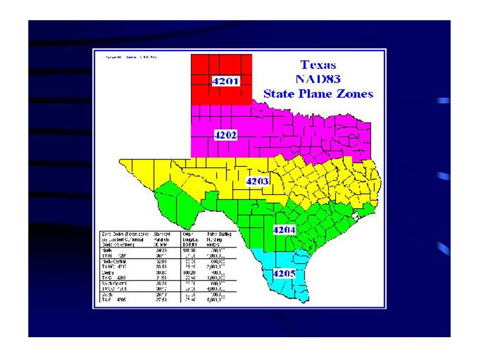


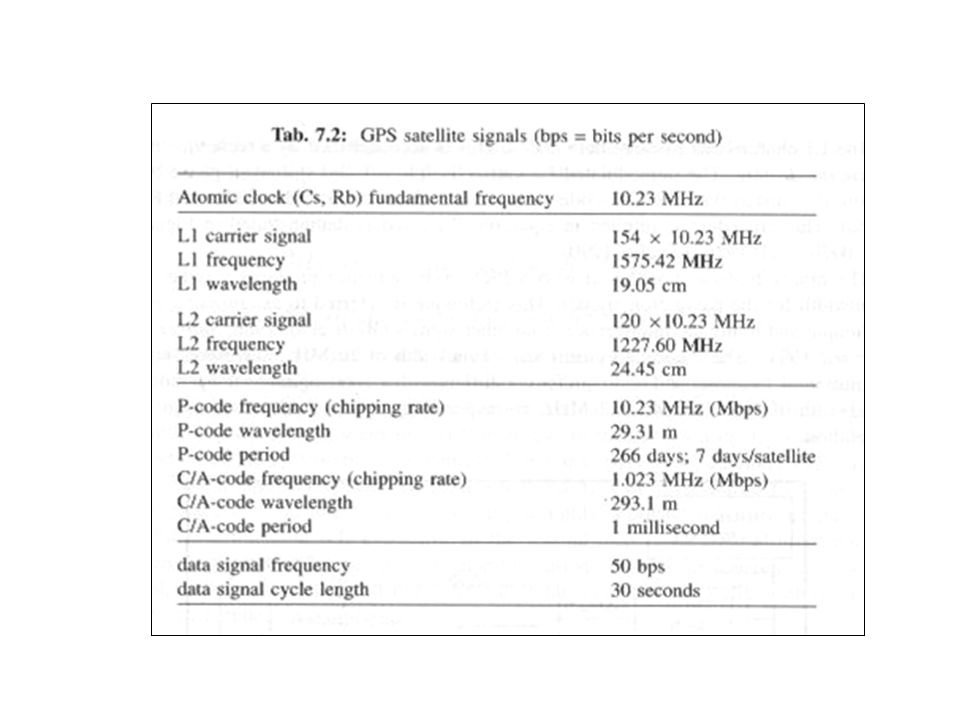


 for Precision Farming>")

 and the Defense Mapping School Reviewed by:____________ Date:_________ Objective:>")


 Dated: 18.11.14 Advance Applications of RS/GIS in Geo-Environmental Conservation Subject Lecture-6.>")


>")

 work>")


