Download presentation
Presentation is loading. Please wait.

1
Step-by-Step Tutorial NEXTA: Simulation Data Visualizer for TRANSIMS
NEXTA: Network EXplorer for Traffic Analysis Sponsored by Federal Highway Administration Developed and Prepared by Dr. Xuesong Zhou, Univ. of Utah Freeware can be downloaded at

2
Sample Occupancy Plot

3
Sample Vehicle Snapshot Plot

4
Sample Bottleneck Snapshot Plot

5
Sample Travel Time Contour (Accessibility) Snapshot Plot
 Snapshot Plot")
6
Tutorial Outline Network and control data visualization
View node and link properties, lane configuration Configure dynamic project menu Time-dependent simulation data visualization View cell occupancy, speed, queue length and vehicle locations, MOE profiles Other tools Find multiple paths Create nodes and links (in development)
")
7
Step 0: Create a Project File
Project file (*.tsp) is used by NEXTA to locate the folder of a TRANSIMS project
 is used by NEXTA to locate the folder of a TRANSIMS project.")
8
Inside a *.tsp Project File
First line should have the relative location of the microsimulation control file Example: TestNet data set setup\master\Microsimulator.ctl Example: Alexandria data set setup\control\Microsimulator.ctl

9
Step 1: Open a Project If the specified microsimulation file is not found in tsp file, the user will be provided with an option to manually load the microsimulation control file, or use the default input file locations

11
Step 1: Open a Project Select iteration number
A user can specify an iteration number for loading average link performance, cell occupancy and vehicle snapshot data. By default, NEXTA automatically identifies and loads the maximum (i.e. the last) iteration number, if multiple iterations of simulation results are available from those files stored in folder “\\results”.
 iteration number, if multiple iterations of simulation results are available from those files stored in folder \\results .")
12
Step 1: Open a Project Define Loading Time Window
For (memory-consuming) cell occupancy and vehicle snapshot data, a user can specify “Start Time” and “End Time” to define a data loading time window to reduce required memory for the GUI program. For link performance data such as density, speed and queue length, NEXTA loads 24 hours of simulation data automatically.
 cell occupancy and vehicle snapshot data, a user can specify Start Time and End Time to define a data loading time window to reduce required memory for the GUI program. For link performance data such as density, speed and queue length, NEXTA loads 24 hours of simulation data automatically.")
13
Input Files Folder Network
Node.txt, Link.txt, Pocket_Lane.txt, Shape.txt, Zone.txt Signalized_Node.txt, Timing_Plan.txt, Phasing_Plan.txt Folder Results Performance.txt (density, speed, queue) Occupancy_Avg.txt (cell occupancy) Snapshot.txt (vehicle locations) Remarks: A test data set with the above files can be downloaded at A user can execute /setup/runall.bat to generate those files
 Occupancy_Avg.txt (cell occupancy) Snapshot.txt (vehicle locations) Remarks: A test data set with the above files can be downloaded at A user can execute /setup/runall.bat to generate those files.")
14
First Look View Tools Distance Move Network Pan Zoom In Zoom Out
Show Entire Network Show/Hide Grid Show/Hide Node Show/Hide Zone

15
Step 2: Zoom In -> View Lane Configuration
Zooming can also be accomplished with the Page Up / Page Down keys, the + / - keys or the mouse wheel.

16
Step 3: Double-Click a Node to Show Node and Control Properties

17
For link 110->105, there are three movements with traffic volume: movement 110->105->104 has 326 vehicles with 729 seconds of average delay, movement 110->105->101 has 323 vehicles with 690 seconds of average delay, and movement 110->105->106 has 896 vehicles with 609 seconds of average delay

18
Step 4: Single-Click a Link to Show Shape Points

19
Step 5: Double-Click a Link to Show Link Property

20
Step 6: Find Node / Find Link / Measure Distance

21
Step 7: Change Color Preferences for Background and Link Types

22
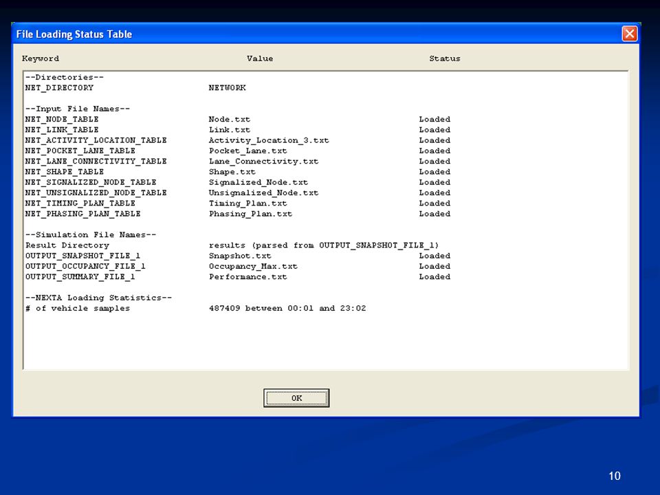
Step 8: View Text File NEXTA fetches input file names directly from the microsimulator control file.

23
Step 9: Select Display Mode to View Simulation Results
Occupancy, Speed, Queue, Vehicles, Volume, Single Vehicle, Travel Time Contour

24
Cell-based Occupancy (I)
")
25
Cell-based Occupancy (II)
")
26
Cell-based Occupancy (III)
")
27
Cell-based Occupancy (IV)
")
28
Speed

29
Queue Length Queue length = average number of stopped vehicles per lane * 7.5 meters

30
Vehicle Vehicle locations are imported from snapshot file

31
Travel Time Contour When the display mode is set to Travel Time Contour Display Mode, the minimum path travel times between a designated destination and other nodes can be plotted on the network window. A user can right-click a node to select menu “Define Destination to Calculate Travel Time Contour”.

32
Travel Time Contour The minimum path travel times between a designated destination and other nodes are plotted on the network window.

33
Travel Time Contour The numbers on a node indicates the calculated minimum path travel time (in minutes) between the current node to the designated destination.
 between the current node to the designated destination.")
34
Travel Time Contour A user can also customizes the thresholds of travel time categories displayed in travel time contour by selecting menu -> View -> Change LOS Interval in Travel Time Contour.

35
Step 10: Show Simulation Results at a Given Time
Simulation Time Clock: 1 hour: 33 min Clock Bar Slider Drag the slider of the clock bar to view simulation results at a given time of simulation horizon

36
Go to First Minute with Vehicles
A user can set the slider of the clock bar at the first minute with vehicles. A snapshot file might only cover a short time period of the entire simulation horizon. After a TRANSIMS project has been loaded, a user can click on menu->View ->Go to First Minute with Vehicles to jump to the first time stamp with snapshot data.

37
Step 11: Play Animation Rewind, play, pause, stop Remarks: Simulation clock is advanced at 1-min interval

38
Step 12: Double-Click a Link to Show MOE Profile
Upstream node -> Downstream node (# link ID) Green line indicates the current simulation time Time axis (unit: min)
 Green line indicates the current simulation time. Time axis (unit: min)")
39
Step 13: Configure MOE Display Dialog
MOE: Density, Speed, Queue Length, Volume Start Time, End Time, Max Y Background color

40
Step 14: Multi-link Comparison
Select multiple links (by using Ctrl+ mouse click) to display MOE time profiles simultaneously for multiple selected links, in the same or different projects. Data can be exported to a CSV file
 to display MOE time profiles simultaneously for multiple selected links, in the same or different projects. Data can be exported to a CSV file.")
41
Step 15: Find Paths Select an origin node,
Right-click to select menu “Define Origin to Find Shortest Path”, Select a destination node, Right-click to select menu “Define Destination to Find Shortest Path”.

42
Step 16: Show Multiple Paths
Path 1: 15 min Path 3: 18.6 min The path finding algorithm uses dynamic travel time calculated from simulated link speed at a given time.

43
Step 17: Create Nodes/Links
Insert node (in the middle of a link) Add one-way link Add two-way link Add zone Add stop sign Add yield sign Add pre-timed controller Add actuated controller Select link type
 Add one-way link. Add two-way link. Add zone. Add stop sign. Add yield sign. Add pre-timed controller. Add actuated controller. Select link type.")
44
Step 18: Show Bottleneck Information
A user can click on menu View->Bottleneck Info-> Bottlenecks to display bottleneck information on different links.

45
Step 18: Show Bottleneck Information

46
Step 19: Sort Link Performance Data
A user can click on menu Project->Sort Link Performance Data to sort, display and export the link performance data in a designated time window. Select an MOE

47
Step 20: Sort Movement Performance Data
A user can click on menu Project->Sort Movement Performance Data to sort, display and export the intersection movement performance data in a designated time window. Select a Field

48
Step 21: Reload Simulation Data with Selected Files
As there might be multiple snapshot files for the same simulation run, a user can click on menu ->File->Reload Simulation Data with Selected Files to reselect the simulation files to be loaded. A user can select the snapshot, performance, and average occupancy files of a designated simulation run individually.

49
Future Development Save network data Run simulation directly
Configure simulation scenarios Use vehicle trajectory information Enable travel time reliability analysis Enable impacted vehicle analysis Identify traffic bottlenecks through vehicle trajectory file

Similar presentations


 with Excel>")


