Download presentation
Presentation is loading. Please wait.

1
Graphical models: approximate inference and learning CA6b, lecture 5

2
Bayesian Networks General Factorization

3
D-separation: Example

4
Trees Undirected Tree Directed TreePolytree

5
Converting Directed to Undirected Graphs (2) Additional links
 Additional links")
6
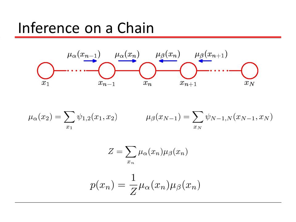
Inference on a Chain

9
Inference in a HMM E step: belief propagation

10
Belief propagation in a HMM E step: belief propagation

11
Expectation maximization in a HMM E step: belief propagation

12
The Junction Tree Algorithm Exact inference on general graphs. Works by turning the initial graph into a junction tree and then running a sum- product-like algorithm.

13
Factor Graphs

14
Factor Graphs from Undirected Graphs

15
The Sum-Product Algorithm (6)
")
18
The Sum-Product Algorithm (5)
")
19
The Sum-Product Algorithm (3)
")
20
The Sum-Product Algorithm (7) Initialization
 Initialization")
22
Sensory observations Prior expectations Forest Tree LeaveRoot Bottom-up Top-down Stem Green Consequence of failing inhibition in hierarchical inference

23
Causal model Pairwise factor graph Bayesian network and factor graph

24
Causal model Pairwise factor graph

25
Causal model Pairwise factor graph

26
Pairwise graphs Log belief ratio Log messages ratio

27
Belief propagation and inhibitory loops - - - - -

28
Tight excitatory/inhibitory balance is required, and sufficient Okun and Lampl, Nat Neuro 2008 Inhibition Excitation

29
Lewis et al, Nat Rev Nsci 05 controls schizophrenia Support for impaired inhibition in schizophrenia See also: Benes, Neuropsychopharmacology 2010, Uhhaas and Singer, Nat Rev Nsci 2010… GAD26

30
Circular inference: Impaired inhibitory loops

31
Circular inference and overconfidence:

32
1 2 32 Renaud Jardri Alexandra Litvinova & Sandrine Duverne The Fisher Task 3 4 A priori Evidence sensorielles Confiance a posteriori

33
Mean group responses Controls:Schizophrenes: Simple Bayes:

34
Control Patients

35
? s SCZ CTL *** * Parameter value (mean + sd) 0.75 0.50 0.25 0.00 Mean parameter values
 Mean parameter values")
36
PANSS positive factor Inference loops and psychosis 25 Non-clinical beliefs (PDI-21 scores) PDI score Strenght of loops
 PDI score Strenght of loops")
37
The Junction Tree Algorithm Exact inference on general graphs. Works by turning the initial graph into a junction tree and then running a sum- product-like algorithm. Intractable on graphs with large cliques.

38
What if exact inference is intractable? Loopy belief propagation works in some scenarios. Markov-Monte-Carlo sampling methods. Variational methods (not covered here)
.")
39
Loopy Belief Propagation Sum-Product on general graphs. Initial unit messages passed across all links, after which messages are passed around until convergence (not guaranteed!). Approximate but tractable for large graphs. Sometime works well, sometimes not at all.
. Approximate but tractable for large graphs. Sometime works well, sometimes not at all..")
45
Neural code for uncertainty: sampling

46
Alternative neural code for uncertainty: sampling Berkes et al, Science 2011

47
Alternative neural code for uncertainty: sampling

48
Learning in graphical models More generally: learning parameters in latent variable models Visible Hidden

49
Learning in graphical models More generally: learning parameters in latent variable models Visible Hidden

50
Learning in graphical models More generally: learning parameters in latent variable models Visible Hidden Huge!

52
Mixture of Gaussians (clustering algorithm) Data (unsupervised)
 Data (unsupervised)")
53
Mixture of Gaussians (clustering algorithm) Data (unsupervised) Generative model: M possible clusters Gaussian distribution
 Data (unsupervised) Generative model: M possible clusters Gaussian distribution")
54
Mixture of Gaussians (clustering algorithm) Data (unsupervised) Generative model: M possible clusters Gaussian distribution Parameters
 Data (unsupervised) Generative model: M possible clusters Gaussian distribution Parameters")
55
Given the current parameters and the data, what are the expected hidden states? Expectation stage: Responsability

56
Given the responsabilities of each cluster, update the parameters to maximize the likelihood of the data: Maximization stage:

57
Learning in hidden Markov models Hidden state Observations cause Forward model Sensory likelihood Inverse model

58
Object present/not Receptor spike/not Time

59
Leak Synaptic input Bayesian integration corresponds to leaky integration.

60
Expectation maximization in a HMM Multiple training sequences: What are the parameters: Transition probabilities Observation probabilities

61
Expectation stage E step: belief propagation

62
Expectation stage E step: belief propagation

63
Expectation stage E step: belief propagation

64
Using “on-line” expectation maximization, a neuron can adapt to the statistics of its input.

65
Fast adaptation in single neurons Adaptation to temporal statistics? Fairhall et al, 2001

Similar presentations


>")


