1. Antennas: from Theory to Practice 5. Popular Antennas
Yi HUANG
Department of Electrical Engineering & Electronics
The University of Liverpool
Liverpool L69 3GJ
This is a general rule, but it may need modification for certain situation.

2. Objectives of this Chapter
To examine and analyse some of the most popular antennas using relevant antenna theories, to see why they have become popular, what their major features and properties (including advantages and disadvantages) are, and how they should be designed.

3. Classification of Antennas
Wire-Type Antennas Aperture-Type Antennas
Dipoles Horn and open waveguide
Monopoles Reflector antennas
Biconical antennas Slot antennas
Loop antennas Microstrip antennas
Helical antennas
Linearly polarised antennas Circularly polarised antennas
Element antennas Antenna array
Narrow-band Broad-band
Transmitting Receiving

4. Evolution of a dipole of total length 2l and diameter d
5.1 Wire Type Antennas
Dipole Antennas
Evolution of a dipole of total length 2l and diameter d

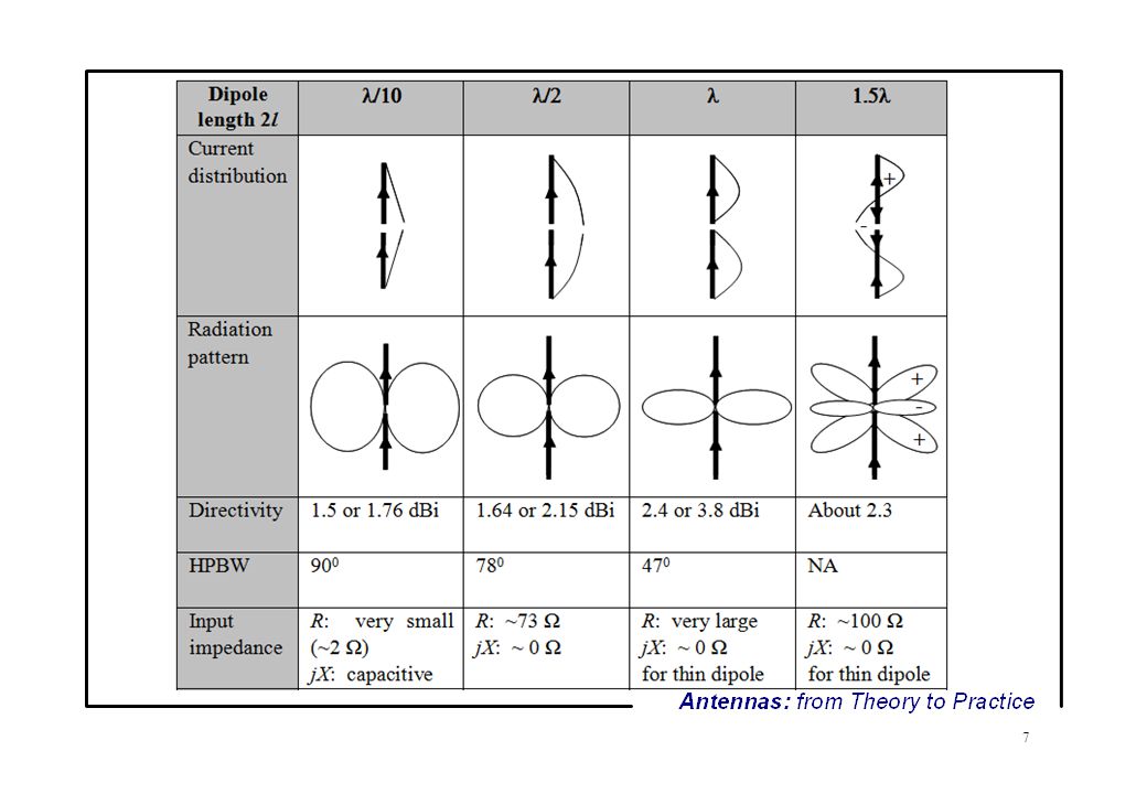
5. Current distribution of dipoles
Current distribution along an open transmission line is:
Thus the current distribution on the dipole is

6. Radiation pattern of dipoles
In the far field:

8. Input impedance of dipoles

9. Electrically short dipoles
When the dipole length is much shorter than a wavelength (< l/10), it can be called an electrically short dipole
The input impedance can be approximated as
Radiation pattern is E() = sin
The directivity is D = 1.5 (1.76dBi)

10. Half-wavelength dipole
The most popular dipole
Radiation pattern: E() = cos[(/2)cos ]/sin
Radiation resistance: 73 
Directivity: (2.15 dBi)
The input impedance is not sensitive to the radius and is about 73 Ω which is well matched with a standard transmission line of characteristic impedance 75 Ω or 50 Ω (with a VSWR < 2).
Its size and radiation pattern are suitable for many applications

11. Example 5.1 Solution on pages 135 - 137
A dipole of the length 2l = 3 cm and diameter d = 2 mm is made of copper wire (s = 5.7  107 S/m) for mobile communications. If the operational frequency is 1 GHz,
a). obtain its radiation pattern and directivity;
b). calculate its input impedance, radiation resistance and radiation efficiency;
c). if this antenna is also used as a field probe at 100 MHz for EMC applications, find its radiation efficiency again, and express it in dB.
Solution on pages

12. Some popular forms of dipole antennas

13. Monopole Antennas Half of a dipole antenna mounted above l
Half of a dipole antenna mounted above
the earth or a ground plane
Normally one-quarter wavelength long
almost the same feature as a dipole,
except the 37 radiation resistance, higher gain, a shorter length, and easier to feed!
Based on the Image Theory
Ground

15. Effects of the ground plane
Its size and material property of can change the radiation pattern (hence the directivity) and input impedance.

16. An example

17. Some popular forms of monopole antennas

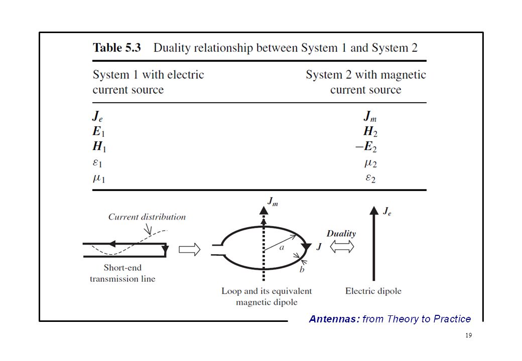
18. Duality Principle System 1 System 2
Duality means the state of combing two different things which are closely linked. In antennas, the duality theory means that it is possible to write the fields of one antenna from the field expressions of the other antenna by interchanging parameters:
System 1
System 2

20. Loop Antennas
For a short dipole
Thus for a small loop

21. Directivity of a loop

22. Current distribution of a resonant loop

23. Radiation pattern of a one wavelength loop – this is very different from that of a short loop!

24. Radiation patterns of loops with various circumferences

25. Input impedance of loops

26. Helical Antennas
It may be viewed as a derivative of the dipole or monopole, but it can also be considered a derivative of a loop.

27. Normal mode Helix
It may be treated as the superposition of n elements, each consisting of a small loop of diameter D and a short dipole of length s, thus the far fields are
They are orthogonal and 90 degrees out of phase;
The combination of them gives a circularly or elliptically polarised wave.
The axial ratio:

28. When the circumference is equal to
the axial ratio becomes unity and the radiation is circularly polarised.

29. Axial Mode Helix
The axial (end-fire) mode occurs when the circumference of the helix is comparable with the wavelength (C = pD ≈ l) and the total length is much greater than the wavelength.
This has made the helix an extremely popular circularly-polarised broadband antenna at the VHF and UHF band frequencies
The recommended parameters for an optimum design to achieve circular polarisation are:

30. The normalised radiation pattern:
Half power beamwidth:
1st null beamwidth:

31. The directivity:
The axial ratio
Radiation resistance

32. Example 5.2
Design a circularly polarised helix antenna of an end-fire radiation pattern with a directivity of 13 dBi. Find out its radiation resistance, HPBW, AR and radiation pattern.
Solution on pages

33. Radiation patterns
Which is better?

34. Yagi-Uda Antennas

35. The driven element (feeder) is the very heart of the antenna
The driven element (feeder) is the very heart of the antenna. It determines the polarisation and centre frequency. For a dipole, the recommended length is about 0.47l to ensuring a good input impedance to a 50 Ω feed line.
The reflector is longer than the feeder to force the radiated energy towards the front. The optimum spacing between the reflector and the feeder is between 0.15 to 0.25 wavelengths.
The directors are usually 10 to 20% shorter than the feeder and appear to direct the radiation towards the front. The director to director spacing is typically 0.25 to 0.35 wavelengths,
The number of directors determines the maximum achievable directivity and gain.

36. Log-periodic Antennas

37. The antenna is divided into the so called active region and inactive regions.
The role of a specific dipole element is linked to the operating frequency: if its length, L, is around half of the wavelength, it is an active dipole and within the active region; Otherwise it is in an inactive region and acts as a director or reflector as in Yagi-Uda antenna
The driven element shifts with the frequency – this is why this antenna can offer a much wider bandwidth than the Yagi-Uda. A travelling wave can also be formed in the antenna.
The highest frequency is basically determined by the shortest dipole length while the lowest frequency is determined by the longest dipole length (L1).

38. Antenna design
This seems to have too many variables. In fact, there are only three independent variables for log-periodic antenna design.
the scaling factor:
the spacing factor:
the apex angle:

40. In practice, the most likely scenario is that the frequency range is given from fmin to fmax, the following equations may be employed for design
Another parameter (such as the directivity or the length of
the antenna) is required to produce an optimised design.

41. Example 5.3 Solution on page 160
Design a log-periodic dipole antenna to cover all UHF TV channels, which is from 470 MHz for channel 14 to 890 MHz for channel 83. Each channel has a bandwidth of 6 MHz. The desired directivity is 8 dBi.
Solution on page 160

42. 5.2 Aperture-Type Antennas
They are often used for higher frequency applications (> 1GHz) than wire-type antennas.

43. Fourier Transform and Radiated Field

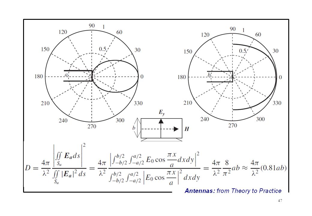
44. How to link the aperture E field to the radiated field
Directivity:

45. Near field and far field

46. Example 5.4 Solution on pages 166 - 168
An open waveguide aperture of dimensions a long x and b along y located in the z = 0 plane. The field in the aperture is TE10 mode and given by
Find
i). the radiated far field and plot the radiation pattern in both the E and H planes;
ii). the directivity.
Solution on pages

48. Horn Antennas
Horn antennas are the simplest and one of the most widely used microwave antennas – the antenna is nicely integrated with the feed line (waveguide) and the performance can be easily controlled.
They are mainly used for standard antenna gain and field measurements, feed element for reflector antennas, and microwave communications.

50. Pyramidal Horn Design
To make this horn, we must have
i.e.

51. The directivity:
We can therefore obtain the design equation
This equation in A can be solved using numerical methods.
For the optimum design, use a first guess approximation

52. Example 5.5 Solution on pages 172 - 173
Design a standard gain horn with a directivity of 20 dBi at 10 GHz. WR-90 waveguide will be used to feed the horn.
Solution on pages

53. Reflector Antennas
Reflector antennas can offer much higher gains than horn antennas and are easy to design and construct.
The most widely used antennas for high frequency and high gain applications in radio astronomy, radar, microwave and millimetre wave communications, and satellite tracking and communications.
The most popular shape is the paraboloid – because of its excellent ability to produce a pencil beam (high gain) with low sidelobes and good cross-polarisation characteristics

54. Paraboloidal and Cassegrain reflector antennas

55. Antenna design
The reflector design problem consists primarily of matching the feed antenna pattern to the reflector. The usual goal is to have the feed pattern about 10 dB down in the direction of the rim, that is the edge taper = (the field at the edge)/(the field at the centre) ≈10 dB.
Directivity:
Half-power beamwidth

56. Offset parabolic reflectors
It reduces aperture blockage while maintaining acceptable structure rigidity

57. Radiation patterns in E and H planes

58. Slots Antennas
They are very low-profile and can be conformed to basically any configuration, thus they have found many applications, for example, on aircraft and missiles.

59. Slot waveguide antenna array: widely used for radar
Equivalent circuit
Slot waveguide antenna array: widely used for radar

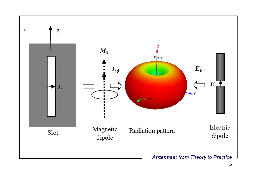
60. Equivalence Principle: for field analysis
The radiated field by the slot is the same as the field radiated by its equivalent surface electric current and magnetic current which were given by
where E and H are the electric and magnetic fields within the slot, and
is the unit vector normal to the slot surface S
For a half-wavelength slot, its equivalent electric surface current JS = ˆn × H = 0, the remaining source at the slot is its equivalent magnetic current MS = −ˆn × E (it would be 2MS if the conducting ground plane were removed using the imaging theory).

62. Babinet’s Principle
The field at any point behind a plane having a screen, if added to the field at the same point when the complementary screen is substituted, is equal to the field at the point when no screen is present.
Apply this to antennas:
Since the impedance for a half-wavelength dipole is about 73 ohms, the corresponding slot has an impedance of

63. Self-complementary antennas – frequency independent
This type of antenna has a constant impedance of

64. Microstrip/Patch Antennas
Ease of construction and integration, relatively low cost, compact low profile configuration and good flexibility
Typical applications for GHz

65. Operational principles
To be a resonant antenna, the length L should be around half of the wavelength. In this case, the antenna can be considered as a l/2 transmission line resonant cavity with two open ends where the fringing fields from the patch to the ground are exposed to the upper half space (z > 0) and are responsible for the radiation.
This radiation mechanism is the same as the slot line, thus there are two radiating slots on a patch antenna.
As a resonant cavity, there are many possible modes (as waveguides), thus a patch antenna is multi-mode and may have many resonant frequencies.

66. Radiation pattern

67. Main properties
Directivity
Input impedance
Bandwidth for VSWR < 2

68. Antenna design
Optimised width:
Resonant freq.:
Length:

69. Example 5.7 Solution on pages 189 - 191
RT/Duroid 5880 substrate ( and d = mm) is to be used to make a resonant rectangular patch antenna of linear polarisation;
a). Design such an antenna to work at 2.45 GHz for Bluetooth applications;
b). Estimate its directivity;
c). If it is to be connected to a 50 ohms microstrip using the same PCB board, design the feed to this antenna;
d). Find the fractional bandwidth for VSWR < 2.
Solution on pages

70. 5.3 Antenna Arrays
Motivations: to achieve desired high gain or radiation pattern, and the ability to provide an electrically scanned beam.
It consists of more than one antenna element and these radiating elements are strategically placed in space to form an array with desired characteristics which are achieved by varying the feed (amplitude and phase) and relative position of each radiating element;
The main drawbacks are the complexity of the feeding network required and the bandwidth limitation (mainly due to the feeding network)

71. A typical antenna array of N elements

72. Pattern Multiplication Principle
Since the total radiated field for an array is the summation of the fields from each element
where An is the amplitude, n is the relative phase, Ee is the radiated field of the antenna element, and AF is called array factor.
Thus the radiation pattern of an array is the product of the pattern of individual element antenna with the (isotropic source) array pattern.

73. Example
Total
array
Total
array
element AF AF
element

74. For a uniform array of a constant d and identical amplitude (say 1)
Thus
The normalised antenna factor of a uniform array:

75. AF: N = 20, d = l and 0 = 0

76. AF: N = 10, d = l and 0 = 0

77. AF: N = 10, d = l/2 and 0 = 0

78. AF for N = 10 and d = l/2, and 0 = 450

79. Phased Array
The maximum of the radiation occurs at  = 0
That is:
Normally the spacing d is fixed for an array, we can control the maximum radiation (or scan the beam) by changing the phase 0 and the wavelength (frequency) – this is the principle of phase/frequency scanned array

80. Broadside and End-fire Arrays
An array is called a broadside array if the maximum radiation of the array is directed normal to its axis (q = 00); while it is called an end-fire array if the maximum radiation is directed along the axis of the array (q = 900).

81. The radiation pattern, SLL, HPBW, and gain for four different source distributions of eight in-phase isotropic sources spaced by l/2; there are trade-offs!

82. Element mutual coupling
The interaction between elements due to their close proximity is called the mutual coupling which affects the current distribution hence the input impedance as well as the radiation pattern
The voltage generated at each element can be expressed as

83. Self-impedance:
Mutual impedance:

84. 5.4 Some Practical Considerations
The differences between transmitting and receiving antennas
From the reciprocity theorem, the field patterns are the same for transmitting or receiving.
Antenna feeding and matching
Balun (a device to connect a balanced antenna to an unbalanced transmission line) may be required.
Polarisation
Polarisation has to be matched from Tx to Rx.
Radomes, housings and supporting structures.
Affecting the antenna performance (impedance, pattern, …)