Download presentation
Presentation is loading. Please wait.

1
Biological Modeling of Neural Networks: Week 11 – Continuum models: Cortical fields and perception Wulfram Gerstner EPFL, Lausanne, Switzerland 11.1 Transients - sharp or slow 11.2 Spatial continuum - model connectivity - cortical connectivity 11.3 Solution types - uniform solution - bump solution 11.4. Perception 11.5. Head direction cells Week 11 – Continuum models –Part 1: Transients

2
Single population full connectivity review from Week 10-part 3: mean-field arguments All neurons receive the same total input current (‘mean field’)
")
3
frequency (single neuron) Homogeneous network All neurons are identical, Single neuron rate = population rate A(t)= A 0 = const Single neuron Review from Week 10: stationary state/asynchronous activity
 Homogeneous network All neurons are identical, Single neuron rate = population rate A(t)= A 0 = const Single neuron Review from Week 10: stationary state/asynchronous activity")
4
All spikes, all neurons fully connected All neurons receive the same total input current (‘mean field’) Index i disappears Week 10-part 3: mean-field arguments
 Index i disappears Week 10-part 3: mean-field arguments")
5
h(t) I(t) ? A(t) potential A(t) t population activity Blackboard: h(t) Week 11-part 1: Transients in a population of uncoupled neurons Students: Which would you choose?
 potential A(t) t population activity Blackboard: h(t) Week 11-part 1: Transients in a population of uncoupled neurons Students: Which would you choose .")
6
Connections 4000 external 4000 within excitatory 1000 within inhibitory Population - 50 000 neurons - 20 percent inhibitory - randomly connected -low rate -high rate input Week 11-part 1: Transients in a population of neurons

7
Population - 50 000 neurons - 20 percent inhibitory - randomly connected 100 200 time [ms] Neuron # 32374 50 u [mV] 100 0 10 A [Hz] Neuron # 32340 32440 100 200 time [ms] 50 -low rate -high rate input Week 11-part 1: Transients in a population of neurons
![Population neurons - 20 percent inhibitory - randomly connected time [ms] Neuron # u [mV] A [Hz] Neuron # time [ms] 50 -low rate -high rate input Week 11-part 1: Transients in a population of neurons](http://images.slideplayer.com/15/4670515/slides/slide_7.jpg "Population neurons - 20 percent inhibitory - randomly connected time [ms] Neuron # u [mV] A [Hz] Neuron # time [ms] 50 -low rate -high rate input Week 11-part 1: Transients in a population of neurons")
8
low noise I(t) h(t) noise-free (escape noise/fast noise) uncoupled population low noise fast transient I(t) h(t) (escape noise/fast noise) high noise slow transient But transient oscillations Week 11-part 1: Theory of transients for escape noise models
 h(t) noise-free (escape noise/fast noise) uncoupled population low noise fast transient I(t) h(t) (escape noise/fast noise) high noise slow transient But transient oscillations Week 11-part 1: Theory of transients for escape noise models")
9
noise model A I(t) h(t) (escape noise/fast noise) high noise slow transient Population activity Membrane potential caused by input blackboard In the limit of high noise, Week 11-part 1: High-noise activity equation
 h(t) (escape noise/fast noise) high noise slow transient Population activity Membrane potential caused by input blackboard In the limit of high noise, Week 11-part 1: High-noise activity equation")
10
noise model A I(t) h(t) (escape noise/fast noise) high noise slow transient Population activity Membrane potential caused by input 1 population = 1 differential equation Week 11-part 1: High-noise activity equation
 h(t) (escape noise/fast noise) high noise slow transient Population activity Membrane potential caused by input 1 population = 1 differential equation Week 11-part 1: High-noise activity equation")
11
Week 10-part 2: mean-field also works for random coupling full connectivityrandom: prob p fixed Image: Gerstner et al. Neuronal Dynamics (2014) random: number K of inputs fixed
 random: number K of inputs fixed.")
12
Quiz 1, now Population equations [ ] A single cortical model population can exhibit transient oscillations [ ] Transients are always sharp [ ] Transients are always slow [ ] in a certain limit transients can be slow [ ] An escape noise model in the high-noise limit has transients which are always slow [ ] A single population described by a single first-order differential equation (no integrals/no delays) can exhibit transient oscillations
![Quiz 1, now Population equations [ ] A single cortical model population can exhibit transient oscillations [ ] Transients are always sharp [ ] Transients are always slow [ ] in a certain limit transients can be slow [ ] An escape noise model in the high-noise limit has transients which are always slow [ ] A single population described by a single first-order differential equation (no integrals/no delays) can exhibit transient oscillations](http://images.slideplayer.com/15/4670515/slides/slide_12.jpg "Quiz 1, now Population equations [ ] A single cortical model population can exhibit transient oscillations [ ] Transients are always sharp [ ] Transients are always slow [ ] in a certain limit transients can be slow [ ] An escape noise model in the high-noise limit has transients which are always slow [ ] A single population described by a single first-order differential equation (no integrals/no delays) can exhibit transient oscillations")
13
Biological Modeling of Neural Networks: Week 11 – Continuum models: Cortical fields and perception Wulfram Gerstner EPFL, Lausanne, Switzerland 11.1 Transients - sharp or slow 11.2 Spatial continuum - from multiple to continuous populations - cortical connectivity 11.3 Solution types - uniform solution - bump solution 11.4. Perception 11.5. Head direction cells Week 11 – part 2 :

14
Blackboard Week 11-part 2: multiple populations continuum

15
Population activity Membrane potential caused by input 1 field = 1 integro-differential equation Week 11-part 2: Field equation (continuum model)
")
16
Exercise 1.1 now (stationary solution) Consider a continuum model, Find analytical solutions: - spatially uniform solution A(x,t)= A 0 Next lecture at 10:45 If done: start with Exercise 1.2 now (spatial stability)
 Consider a continuum model, Find analytical solutions: - spatially uniform solution A(x,t)= A 0 Next lecture at 10:45 If done: start with Exercise 1.2 now (spatial stability)")
17
Week 11-part 2: coupling across continuum xy Mexican hat

18
Week 11-part 2: cortical coupling

19
Biological Modeling of Neural Networks: Week 11 – Continuum models: Cortical fields and perception Wulfram Gerstner EPFL, Lausanne, Switzerland 11.1 Transients - sharp or slow 11.2 Spatial continuum - from multiple to continuous populations - cortical connectivity 11.3 Solution types - uniform solution - bump solution 11.4. Perception 11.5. Head direction cells Week 11 – part 3 :

20
Week 11-part 3: Solution types (ring model) Coupling: Input-driven regime Bump attractor regime
 Coupling: Input-driven regime Bump attractor regime")
21
0 A(x) I. Edge enhancement Weaker lateral connectivity I(x) Possible interpretation of visual cortex cells: (see final part this week) Field Equations: Wilson and Cowan, 1972 Week 11-part 3: Solution types: input driven regime
 Possible interpretation of visual cortex cells: (see final part this week) Field Equations: Wilson and Cowan, 1972 Week 11-part 3: Solution types: input driven regime.")
22
0 A II: Bump formation: activity profile in the absence of input strong lateral connectivity Possible interpretation of head direction cells: (see later today) Field Equations: Wilson and Cowan, 1972 Week 11-part 3: Solution types: bump solution
 Field Equations: Wilson and Cowan, 1972 Week 11-part 3: Solution types: bump solution")
23
Exercise 2.1+2.2 now (stationary bump solution) Consider a continuum model, Find analytically the bump solutions w(x-y) Next lecture at 11:28
 Consider a continuum model, Find analytically the bump solutions w(x-y) Next lecture at 11:28")
24
Continuum: stationary profile Comparison simulation of neurons and macroscopic field equation Spiridon&Gerstner See: Chapter 9, book: Spiking Neuron Models, W. Gerstner and W. Kistler, 2002 Week 11-part 3: Solution types: bump solution

25
Week 11-part 3: Solution types (continuum model) time
 time")
26
Biological Modeling of Neural Networks: Week 11 – Continuum models: Cortical fields and perception Wulfram Gerstner EPFL, Lausanne, Switzerland 11.1 Transients - sharp or slow 11.2 Spatial continuum - model connectivity - cortical connectivity 11.3 Solution types - uniform solution - bump solution 11.4. Perception 11.5. Head direction cells Week 11 – part 4:

27
Basic phenomenology 0 A(x) I. Edge enhancement Weaker lateral connectivity I(x) Possible interpretation of visual cortex cells: contrast enhancement in - orientation - location Field Equations: Wilson and Cowan, 1972 Week 11-part 5: uniform/input driven solution
 Possible interpretation of visual cortex cells: contrast enhancement in - orientation - location Field Equations: Wilson and Cowan, 1972 Week 11-part 5: uniform/input driven solution.")
28
Continuum models: grid illusion

29
Continuum models: Mach Bands

30
Week 11-part 4: Field models and Perception

33
Biological Modeling of Neural Networks: Week 11 – Continuum models: Cortical fields and perception Wulfram Gerstner EPFL, Lausanne, Switzerland 11.1 Transients - sharp or slow 11.2 Spatial continuum - model connectivity - cortical connectivity 11.3 Solution types - uniform solution - bump solution 11.4. Perception 11.5. Head direction cells Week 11 – part 5:

34
Basic phenomenology 0 A II: Bump formation strong lateral connectivity Possible interpretation of head direction cells: always some cells active indicate current orientation Week 11-part 5: Bump solution

35
rat brain CA1 CA3 DG pyramidal cells soma axon dendrites synapses electrode Place fields Week 11-part 5: Hippocampal place cells

36
Main property: encoding the animal’s location place field Week 11-part 5: Hippocampal place cells

37
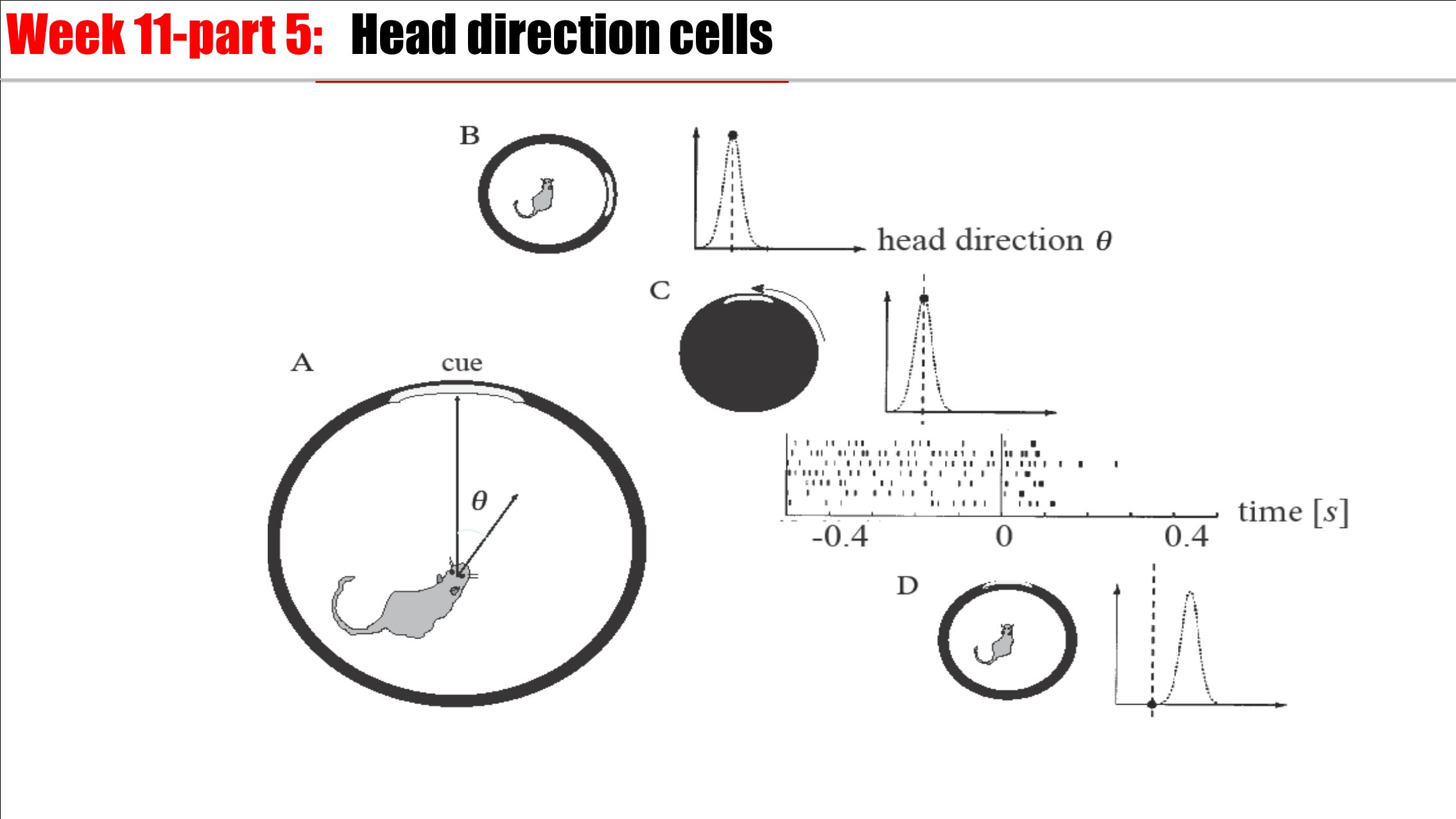
Main property: encoding the animal ’s heading Preferred firing direction r ( i i Week 11-part 5: Head direction cells

38
Main property: encoding the animal ’s allocentric heading Preferred firing direction r ( i i 0 90 180 270 300 Week 11-part 5: Head direction cells

40
11.1 Transients - sharp or slow 11.2 Spatial continuum - model connectivity - cortical connectivity 11.3 Solution types - uniform solution - bump solution 11.4. Perception 11.5. Head direction cells Week 11-Continuum models The END

Similar presentations


, Ch 2http://www.nordita.dk/~mulvad/Thesis.>")


 Lecture 12 Course: Neural Networks and Biological Modeling Wulfram.>")


