Download presentation
Presentation is loading. Please wait.

1
Using a Coupled Groundwater-Flow and Nitrate-Balance-Regression Model to Explain Trends, Forecast Loads, and Target Future Reclamation Ward Sanford, USGS, Reston, Virginia Jason Pope, USGS, Richmond, Virginia David Selnick, USGS, Reston, Virginia

2
Objectives: To develop a groundwater flow model that can simulate return-times to streams (base-flow ages) on the Delmarva Peninsula To explain the spatial and temporal trends in nitrate on the Delmarva Peninsula using a mass-balance regression equation that includes the base-flow age distributions obtained from the flow model To use the calibrated equation to forecast total nitrogen loading to the Bay from the Eastern Shore To forecast changes in future loadings to the bay given different loading application rates at the land surface To develop maps that will help resource managers target areas that will respond most efficiently to better management practices

3
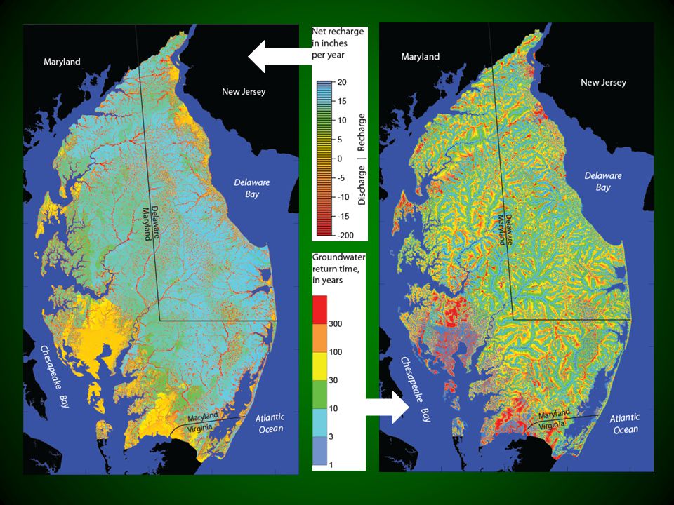
Ground-Water Model of the Delmarva Peninsula
MODFLOW 2005 500 ft cell resolution 7 Model Layers 4+ million active cells 30-m DEM, LIDAR 300 ft deep Steady State Flow MODPATH travel times

5
Groundwater Level Observations Groundwater Age Observations

7
Age Histograms of two of the Real-Time Watersheds

8
substantial stream nitrate Data and were used: Morgan Creek
Seven watersheds had substantial stream nitrate Data and were used: Morgan Creek Chesterville Branch Choptank River Marshyhope Creek Nanticoke River Pocomoke River Nassawango Creek 1 2 3 4 5 6 7

9
Low flow High flow

10
Nitrate Mass-Balance Regression Equation
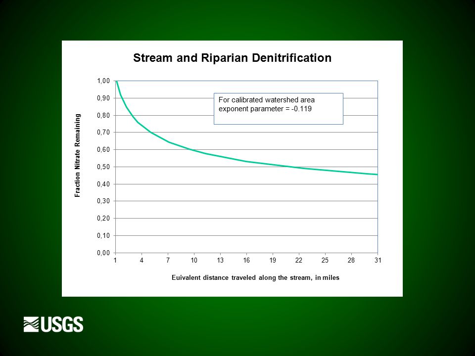
Simulated surface water concentration in stream Soil Term Riparian Term Non-ag Term Pre-ag Term = Concentration below ag field X X X X – RL Denitrification Dilution Simulated groundwater concentration in ag field well Concentration below ag field Soil Term = X – RL FUE & PUE =Fertilizer and Poultry Uptake Efficiencies { [ ] [ ] } Concentration below ag field Recharge Rate Fertilizer Load 1 - Poultry Load = X X FUE 1 - + X PUE Soil Term = (S/5)m = (AREA)n Riparian Term S = soil drainage factor AREA is for the watershed In square miles
m. = (AREA)n. Riparian. Term. S = soil drainage. factor. AREA is for the watershed. In square miles.")
13
Soil Factor (S) in Equation:
Very poorly drained Somewhat poorly drained Poorly drained Moderately well drained Well drained Somewhat excessively drained Excessively drained

15
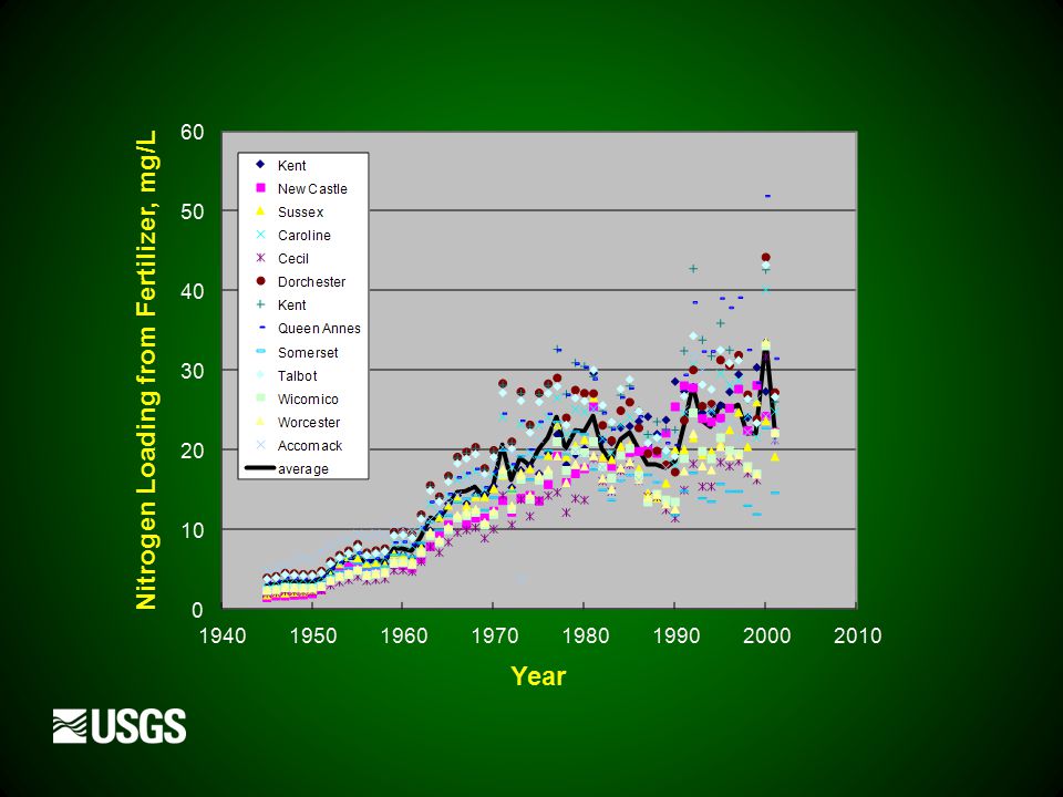
Fertilizer Uptake Efficiency Manure Uptake Efficiency
Regression Number Fertilizer Uptake Efficiency Manure Uptake Efficiency Percent Increase in Uptake Efficiencies Riparian and Stream Denitrificaiton loss exponent Soil Deintirficaiton loss exponent Number of Parameters estimated Sum of Squared Weighted Residuals Standard Error of Regression 1 83% 2 8388 122 82% 70% 0.670 3 5834 85 72% 63% -0.152 3698 54 4 74% 36% -0.146 0.425 2540 37 5 67% 40% 24% -0.114 0.566 2181 33 10% upper parameter value limit 62% -0.110 0.8 10% lower parameter value limit 64% 32% 12% -0.140 0.2 10% limits as percent of value 3% 25% 58% 13% 80%

16
Best Fit for Four Parameters
with best-fit changes in Fertilizer and Uptake Efficiences

17
Groundwater Discharge
Stream Hydrograph Surface Runoff Component Groundwater Discharge Component FLOW RATE HIGH N FLOW LTMDFR X 1.4 Long-Term Mean Daily Flow Rate (LTMDFR) Low N flow High N flow LOW N FLOW Graphical Hydrograph Separation TIME For the Real-time watersheds, the fraction of the water that discharges above the High/Low N cutoff correlates very well to the fraction of the total streamflow that is either surface runoff or that which the model calculates as quickly rejected recharge. Also for the real-time watersheds, the flux-weighted concentration of nitrate in the high-flow section was consistently equal to about 65% of the low-flow concentration. These factors combined allow for BOTH a low-flow and high-flow nitrogen flux to be calculated from all of the other watersheds and for the entire Eastern Shore as a whole.
 Low N flow. High N flow. LOW N. FLOW. Graphical Hydrograph. Separation. TIME For the Real-time watersheds, the fraction of the water that discharges above. the High/Low N cutoff correlates very well to the fraction of the total streamflow. that is either surface runoff or that which the model calculates as quickly rejected recharge. Also for the real-time watersheds, the flux-weighted concentration of nitrate in the. high-flow section was consistently equal to about 65% of the low-flow concentration. These factors combined allow for BOTH a low-flow and high-flow nitrogen flux to be calculated from all of the other watersheds and for the entire Eastern Shore as a whole.")
20
EPA Targets

21
Targeting of HUC-12 Watersheds by Average Nitrate Yield
Average nitrate yield to local stream >5 mg/L 5 mg/L 4 mg/L 3 mg/L 2 mg/L 1 mg/L <1 mg/L or outside Bay watershed

22
Targeting that Includes Response Time
and Nitrogen Delivered to the Bay Targeting Matrix Nitrate Concentration < 4 mg/L 5 - 7 mg/L >7 mg/L < 7 yrs yrs > 20 yrs Groundwater Return Time

23
Targeting that Includes Response Time
and Nitrogen Delivered to the Bay Targeting Matrix Nitrate Concentration < 4 mg/L 5 - 7 mg/L >7 mg/L < 7 yrs yrs > 20 yrs Groundwater Return Time >3 mg/L

24
From: USGS NAWQA Cycle 3 Planning Document--unpublished

25
Summary and Conclusions
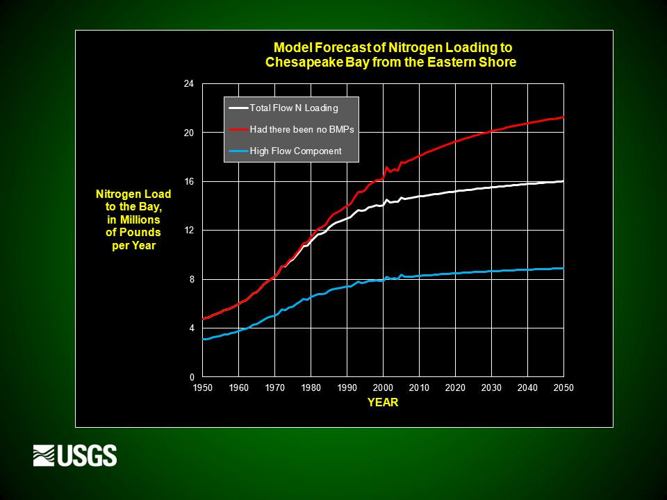
Results from a groundwater flow model were coupled to a nitrate-mass-balance regression model and calibrated against stream nitrate data. The calibrated model suggests that nitrogen uptake efficiencies on the Eastern Shore may be improving over time. EPA targets for reduced loading of 3 million pounds on the Eastern Shore per year will not likely be reasonably reached for several decades, much less by 2020, even with severe cutbacks in fertilizer use The model can help target areas where reduced nitrogen loadings would be the most beneficial at reducing total loadings to the Bay.

Similar presentations


>")


 Tripathy ABE 527 (Spring’ 04)>")


