1. The Problems of Electric Polarization
Tutorial lecture 1 in Kazan Federal University
The Problems of Electric Polarization
Dielectrics in Static Field
Yuri Feldman

2. Ancient times
1745 first condenser constructed by Cunaeus and Musschenbroek
And is known under name of Leyden jar
1837 Faraday studied the insulation material,which he called the dielectric
Middle of 1860s Maxwell’s unified theory of electromagnetic phenomena
1847 Ottaviano-Fabrizio Mossotti
 = n2
1879 Clausius

3. 1887 Hertz
1897 Drude
Lorenz
1912 Debye
Internal field
Dipole moment
Robert Cole

4. Dielectric response on mesoscale
Dielectric spectroscopy is sensitive to relaxation processes
in an extremely wide range of characteristic times ( s)
Broadband Dielectric Spectroscopy
Time Domain Dielectric Spectroscopy; Time Domain Reflectometry
10-6
10-4
10-2
102
104
106
108
1010
1012
f (Hz)
Macromolecules
Glass forming
liquids
Porous materials
and colloids
Clusters
Single droplets
and pores
Water
ice

5. Broadband Dielectric Spectroscopy Time Domain Dielectric Spectroscopy
Dielectric response in biological systems
Dielectric spectroscopy is sensitive to relaxation processes
in an extremely wide range of characteristic times ( s)
Broadband Dielectric Spectroscopy
Time Domain Dielectric Spectroscopy
10-1
101
102
103
104
105
106
107
108
109
1010
1011
1012
ice H 
H3N+ — C — COO- R
f (Hz)
Cells
Proteins
Water
Ala Asp Arg Asn
Cys Glu Gln His
Ile Leu Lys Met
Phe Ser Thr Trp
Tyr Val
Amino acids
DNA, RNA
P - N+
Head group
region
Lipids
Tissues
-Dispersion
 - Dispersion
 - Dispersion
 - Dispersion

6. Electric dipole - definition
The electric moment of a point charge relative to a fixed point is defined as er, where r is the radius vector from the fixed point to e. Consequently, the total dipole moment of a whole system of charges ei relative to a fixed origin is defined as:
A dielectric substance can be considered as consisting of elementary charges ei , and
if it contains no net charge.
If the net charge of the system is zero, the electric moment is independent of the choice of the origin: when the origin is displaced over a distance ro, the change in m is given by: 6

7. Thus m equals zero when the net charge is zero.
Then m is independent of the choice of the origin. In this case equation (1.1) can be written in another way by the introduction of the electric centers of gravity of the positive and the negative charges.
These centers are defined by the equations:
and
in which the radius vectors from the origin to the centers are represented by rp and rn respectively and the total positive charge is called Q. 7

8. The difference rp-rn is equal to the vector distance between the centers of gravity, represented by a vector a, pointing from the negative to the positive center ( Fig.1).
Thus we have:
Therefore the electric moment of a system of charges with zero net charge is generally called the electric dipole moment of the system.
A simple case is a system consisting of only two point charges + e and - e at a distance a.
Such a system is called a (physical) electric dipole, its moment is equal to ea, the vector a pointing from the negative to the positive charge.
Under the influence of the external electrical field, the positive and negative charges in the particle are moved apart: the particle is polarized. In general, these induced dipoles can be treated as ideal; permanent dipoles, however, may generally not be treated as ideal when the field at molecular distances is to be calculated. 8

9. The values of molecular dipole moments are usually expressed in Debye units. The Debye unit, abbreviated as D, equals electrostatic units (e.s.u.).
The permanent dipole moments of non-symmetrical molecules generally lie between 0.5 and 5D. It is come from the value of the elementary charge eo that is 4.410-10 e.s.u. and the distance s of the charge centers in the molecules amount to about cm.
In the case of polymers and biopolymers one can meet much higher values of dipole moments ~ hundreds or even thousands of Debye units. To transfer these units to SI system one have to take into account that 1D=3.310-30 coulombsm. 9

10. Deformation polarization
Types of polarization
Deformation polarization
a. Electron polarization - the displacement of nuclear and electrons in the atom under the influence of external electric field. As electrons are very light they have a rapid response to the field changes; they may even follow the field at optical frequencies. + - + - + -
Electric Field
b. Atomic polarization - the displacement of atoms or atom groups in the molecule under the influence of external electric field. 10

11. Orientation polarization:
The electric field tends to direct the permanent dipoles.

12. Ionic Polarization
In an ionic lattice, the positive ions are displaced in the direction of the applied electric field whilst the negative ions are displaced in the opposite direction, giving a resultant dipole moment to the whole body. - + - + - - - - + - + + + + - - + - - - - - - + + + + - + + + + - - + - - - + - - - + + + + + +
Electric field 12

13. The vector fields E and D.
For measurement inside matter, the definition of E in vacuum, cannot be used.
There are two different approaches to the solution of the problem how to measure E inside matter. They are:
1. The matter can be considered as a continuum in which, by a sort of thought experiment, virtual cavities were made. (Kelvin, Maxwell). Inside these cavities the vacuum definition of E can be used.
2. The molecular structure of matter considered as a collection of point charges in vacuum forming clusters of various types. The application here of the vacuum definition of E leads to a so-called microscopic field (Lorentz, Rosenfeld, Mazur, de Groot). If this microscopic field is averaged, one obtains the macroscopic or Maxwell field E .

14. For the solution of this problem of how to determine the electric field inside matter, it is also possible first to introduce a new vector field D in such a way that for this field the source equation will be valid.
The main problem of physics of dielectrics is passing from a phenomenological macroscopic linear dielectric response to the microscopic structure in terms of electrons, nuclei, atoms, molecules and ions. In general case the problem is still unresolved completely.
According to Maxwell, matter is regarded as a continuum. To use the definition of the field vector E, a cavity has to be made around the point where the field is to be determined.
However, the force acting upon a test point charge in this cavity will generally depend on the shape of the cavity, since this force is at least partly determined by effects due to the walls of the cavity. This is the reason that two vector fields defined in physics of dielectrics:
The electric field strength E satisfying curlE=0, and the dielectric displacement D, satisfying div D=4.

15. where P called the POLARIZATION.
The Maxwell continuum can be treated as a dipole density of matter. Difference between the values of the field vectors arises from differences in their sources. Both the external charges and the dipole density of the piece of matter act as sources of these vectors.
The external charges contribute to D and to E in the same manner. Because of the different cavities in which the field vectors are measured, the contribution of dipole density to D and E are not the same. It can be shown that
where P called the POLARIZATION.
Generally, the polarization P depends on the electric strength E. The electric field polarizes the dielectric.
The dependence of P on E can take several forms: 15

16. The polarization proportional to the field strength
The polarization proportional to the field strength. The proportional factor  is called the dielectric susceptibility.
in which  is called the dielectric permittivity. It is also called the dielectric constant, because it is independent of the field strength. It is, however, dependent on the frequency of applied field, the temperature, the density (or the pressure) and the chemical composition of the system.
Dielectric sample E D

17. Polar and Non-polar Dielectrics
To investigate the dependence of the polarization on molecular composition, it is convenient to assume the total polarization P to be divided into two parts: the induced polarization P caused by the translation effects, and the dipole polarization P caused by the orientation of the permanent dipoles.
A non-polar dielectric is one whose molecules possess no permanent dipole moment.
A polar dielectric is one in which the individual molecules possess a dipole moment even in the absence of any applied field (i.e. the center of positive charge is displaced from the center of negative charge). 17

18. Induced and orientation polarizations Orientation polarization
Induced polarization
Nk is the number of particles per volume unit;
 is the scalar polarizability of a particle ;
Ei is the Internal Field, the average field strength acting upon that particle. It is defined as the total electric field at the position of the particle minus the field due to the particle itself.
k is the index referred to the k-th kind of particle.
is the value of the permanent dipole vector
averaged over all orientations. 18

19. Orientation polarization, Average dipole moment
The energy of the random oriented permanent dipole  in the electric field dependent on the part of the electric field tending to direct the permanent dipoles. This part of the field is called the directing field Ed.
Averaging E 
The relative probabilities of the various orientations of dipole depend on this energy according to Boltzmann’s distribution law:

20. L(a) is called Langeven function
where
and
In Fig. the Langeven function L(a) is plotted against a. L(a) has a limiting value 1, which was to be expected since this is the maximum of cos. For small values of a, <cos> is linear in Ed: 20

21. The approximation of may be used as long as
At room temperature (T=300o K) this gives for a dipole of 4D:
= v/cm
For a value of  smaller than the large value of 4D, the value calculated for Ed is even larger. In usual dielectric measurements, Ed is much smaller than 105 v/cm and the use of is allowed.
From the linear response approximation it follows that:
Substituting this into the main relationship for the orientation polarization, we get: 21

22. Fundamental equation
This is the fundamental equation is the starting point for expressing Ei and Ed as functions of the Maxwell field E and the dielectric constant .

23. and electrostatic problems
Dipole moments
and electrostatic problems
Let us put a dielectric sphere of radius a and dielectric constant 2, in a dielectric extending to infinity (continuum), with dielectric constant 1, to which an external electric field is applied.
Outside the sphere the potential satisfies Laplace's equation =0, since no charges are present except the charges at a great distance required to maintain the external field. On the surface of the sphere Laplace's equation is not valid, since there is an apparent surface charge.
Inside the sphere, however, Laplace's equation can be used again. Therefore, for the description of , we use two different functions, 1 and 2, outside and inside the sphere, respectively. 23

24. Let us consider the center of the sphere as the origin of the coordinate system, we choose z-axis in the direction of the uniform field. Following relation in the terms of Legendre polynomial represents the general solution of Laplace’s equation:
The boundary conditions are: 1.
Since  is continuous across a boundary 2.
since the normal component of D must be continuous at the surface of the sphere 3. 4.
At the center of the sphere (r=0) 2 must not have a singularity.

25. A spherical cavity in dielectric
The total field E2 inside the sphere is accordingly is given by:
A spherical cavity in dielectric
In the special case of a spherical cavity in dielectric (1=; 2=1), equation is reduced to:
2=1
1=
This field is called the "cavity field". The lines of dielectric displacement given by Dc=3Do/(2+1) are more dens in the surrounding dielectric, since D is larger in the dielectric than in the cavity 25

26. A dielectric sphere in vacuum
For a dielectric sphere in a vacuum (1=1; 2=), the equation is reduced to:
where E is the field inside the sphere.
The density of the lines of dielectric displacement Ds is higher in the sphere than in the surrounding vacuum, since inside the sphere Ds=3Eo/(+2). Consequently, it is larger than Eo.
1=1
2=
The field outside the sphere due to the apparent surface charges is the same as the field that would be caused by a dipole m at the center of the sphere, surrounded by a vacuum, and given by:

27. Type of interactions Two types of interaction forces:
-Short range forces- interaction between nearest neighbors:
Chemical bonds,
Van der Waals attraction,
Repulsion forces,
etc.
Long rang dipolar interaction forces
Dipole-dipole interaction
Dipole -charge interaction
Due to the long range of the dipolar forces an accurate calculation of the interaction of a particular dipole with all other dipoles of a specimen would be very complicated.
The different approaches where developed for solving this problem.

28. Lorentz’s method 28

29. Non-polar dielectrics. Lorentz's field. Clausius-Massotti formula.
The apparent surface charges
For a non-polar system the fundamental equation for the dielectric permittivity (2.49) is simplified to:  E
Real cavity  E
Virtual cavity _ +
In this case, only the relation between the internal field and the Maxwell field has to be determined. Let us use the Lorentz approach in this case. He calculated the internal field in homogeneously polarized matter as the field in a virtual spherical cavity.
Lorentz’s field
Lines of dielectric displacement

30. For a pure compound (k=1)
Clausius-Massotti formula

31. Debye theory; Gases and polar molecules in non-polar solvent
But in many cases, however, the Debye equation is in considerable disagreement with the experiment. It works very nice for gases at normal pressures. In this case one has -1<<1 and equation can be written as:
This is generally called the Debye equation. It was the first relationship that made the connection between the molecular parameter of the substance being tested and the phenomenological (macroscopic) parameter that can be experimentally measured. 31

32. The reaction field and Onsager’s approach
When a molecule with permanent dipole strength  is surrounded by other particles, the inhomogeneous field of the permanent dipole polarizes its environment. In the surrounding particles moments proportional to the polarizability are induced, and if these particles have a permanent dipole moment their orientation is influenced. To calculate this effect one can use a simple model: an ideal dipole in a center of a spherical cavity.
The inhomogeneous field of the permanent dipole
Electric dipole field lines
Line of force in the dipole field 32

33. The reaction field of a non-polarizable point dipole
Let us assume that only one kind of molecule is presented and a is value approximately equal to what is generally considered to be the “molecular radius”
Solving the Laplace equation with slightly different boundary conditions : 1. 2. 3.
We can calculate:
The field in the cavity is a superposition of the dipole field in vacuum and a uniform field R, given by:
and the factor of the reaction field is equal to 33

34. The reaction field of a polarized point dipole
Formally, the field of dielectric can be described as the field of a virtual dipole c at the center of the cavity, given by:
The presented model involves a number of simplifications, since the dipole is assumed to be ideal and located at the center of the molecule, which is supposed to be spherical and surrounded by a continuous dielectric.
The reaction field of a polarized point dipole
In this case the permanent dipole has an average polarizability , and therefore the reaction field R induces a dipole R and satisfies the equation:
Under the influence of the reaction field the dipole moment is increased considerably, the increased moment is:

35. Considering
We can obtain that
In the case of polar dielectrics, the molecules have a permanent dipole moment , and both parts of the fundamental must be taken into account.
In the case of non-polar liquids the internal field can be considered as the sum of two parts; one being the cavity field and another the reaction field of the dipole induced in the molecule Ei=Ec+R.

36. For polar molecules the internal field can also built up from the cavity field and the reaction field, taking into account now the reaction field of the total dipole moment of the molecule.  z 
The angle between the reaction field of the permanent part of the dipole moment and the permanent dipole moment itself will be constant during the movements of the molecule.
It means that in a spherical cavity the permanent dipole moment and the reaction field caused by it will have the same direction. Therefore, this reaction field R does not influence the direction of the dipole moment of the molecule under consideration, and does not contribute to the directing field Ed.
On the other hand, the reaction field does contribute to the internal field Ei, because it polarizes the molecule. As a result, we find a difference between the internal field Ei and the directing field Ed.

37. Since the reaction field R belongs to one particular orientation of the dipole moment, the difference between Ei and Ed will give by the value of the reaction field averaged over all orientations of the polar molecule: z 
The direction field Ed can be obtained by the following procedure:  
) remove the permanent dipole of a molecule without changing its polarizability;
) let the surrounding dielectric adapt itself to the new situation;
) then fix the charge distribution of the surroundings and remove the central molecule.
The average field in the cavity so obtained is equal to the value of Ed that is to be calculated, since we have eliminated the contribution of R to Ei by removing the permanent dipole of the molecule.

38. This equation is generally called the Onsager equation
This equation is generally called the Onsager equation. It makes possible the computation of the permanent dipole moment of a molecule from the dielectric constant of the pure dipole liquid if the density and  are known.

39. Relationships between the different kinds of electric fields
In this case of the internal field can be considered as the sum of two parts; one being the cavity field and another that is the reaction field of the dipole induced in the molecule:
The non-polar liquids
In order to describe polarization of matter the different kinds of electric fields where introduced : Maxwell’s field E ; internal field Ei ; Lorentz field EL ; direction field Ed reaction field R and the cavity field EC
Polar molecules
For polar molecules the internal field can also built up from the cavity field and the reaction field, taking into account now the reaction field of the total dipole moment of the molecule.
Since the reaction field R belongs to one particular orientation of the dipole moment, the difference between Ei and Ed will give by the value of the reaction field averaged over all orientations of the polar molecule:
Let us consider the relationships between these
fields in the different systems.
Gases and polar molecules in non-polar solvent

40. The Kirkwood –Froehlich approach
In the above approximations we considered non-polar systems, polar dilute systems and polar systems without short range interactions. In all these cases the dipole-dipole interactions between molecules where not taking into account.
A more general theory was developed by Kirkwood and subsequently refined by Froehlich. This approach takes into account the dipole-dipole interactions, which appears in a more dense state under the influence of the short range interactions 40

41. N-N molecules are considered to form a continuum
In this case the external field working in the sphere is the cavity field
N dipoles i
E is the Maxwell field in the material outside the sphere
Here n=N /V is the number density, and the tensor A plays the role of a polarizability;
N-N molecules are considered to form a continuum
For non polarizable molecules

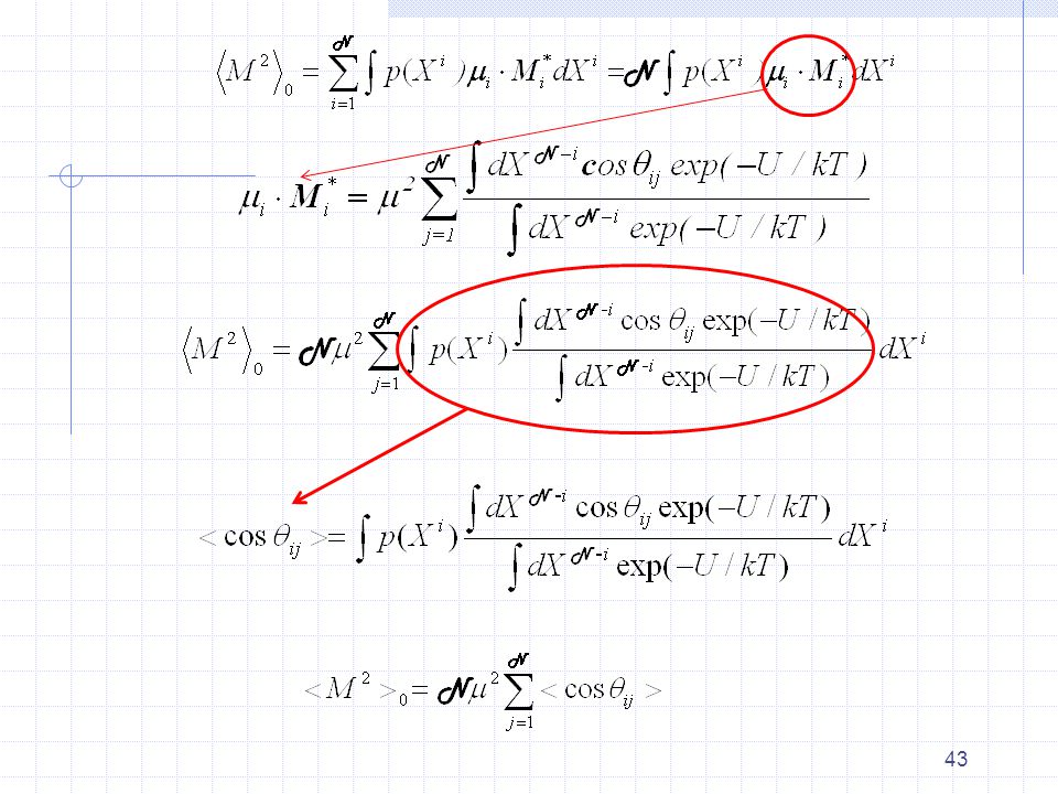
42. In this equation the superscript N to dX to emphasize that the integration is performed over the positions and orientations of N molecules (here dX=r2sindrdd, is the expression for a volume element in spherical coordinates).
Since i is a function of the orientation of the i-th molecule only, the integration over the positions and orientations of all other molecules, denoted as N -i, can be carried out first. In this way we obtain (apart from a normalizing factor) the average moment of the sphere in the field of the i-th dipole with fixed orientation. The averaged moment, denoted by Mi*, can be written as:
N dipoles i
The average moment Mi* is a function of the position and orientation of the i-th molecule only.
Denoting the position and orientation coordinates of the i-th molecule by Xi and using a weight factor p(Xi)

44. The left part of the Onsager equation for the non polarized molecules
The deviations of Mi* from the value i are the result of molecular interactions between the i-th molecule and its neighbors.
It is well known that liquids are characterized by short-range order and long-range disorder. The correlations between the orientations (and also between positions) due to the short-range ordering will lead to values of Mi* differing from i. This is the reason that Kirkwood introduced a correlation factor g which accounted for the deviations of
from the value 2:

45. When there is no more correlation between the molecular orientations than can be accounted for with the help of the continuum method, one has g=1 we are going to Onsager relation for the non-polarizable case, for rigid dipoles with =1.
An approximate expression for the Kirkwood correlation factor can be derived by taking only nearest-neighbors interactions into account. In that case the sphere is shrunk to contain only the i-th molecule and its z nearest neighbors. We then have:
Since after averaging the result of the integration will be not depend on the value of j, all terms in the summation are equal and we may write:
with N=z+1.

46. Approximation of Fröhlich
 g will be different from 1 when <cosij>0, i.e. when there is correlation between the orientations of neighboring molecules.
When the molecules tend to direct themselves with parallel dipole moments, <cosij> will be positive and g>1.
When the molecules prefer an ordering with anti-parallel dipoles, g <1.
Approximation of Fröhlich 

47. Main relationships in static dielectric theory
Clausius-Mossotti equation
Non-polar systems
Debye equation
Polar diluted systems
Onsager Equation
Polar systems 
Polar systems, short range interactions
Kirkwood-Fröhlich equation