1. Minimal Models for Quantum Decoherence in Coupled Biomolecules
Joel Gilmore
Ross H. McKenzie
University of Queensland, Brisbane, Australia
Gilmore and McKenzie, J. Phys.:Cond. Matt. 17, 1735 (2005)
and quant-ph/ , to appear in Chem. Phys. Lett

2. Why should biologists be interested in quantum?
Why should physicists be interested in biology?
Quantum mechanics plays a critical role in much of biology!
They’re all highly efficient, highly refined, self assembling quantum nanoscale devices.
Retinal, responsible for vision
Ultrafast vision receptor
Light harvesting complexes in photosynthesis
Ultraefficient collection & conversion of light
Green Fluorescent Protein
Highly efficient marker
The first question you might ask, is why should a biologist be interested in quantum mechanics? After all, most biologists don’t know or care about field theory or the Schrodinger equation and get along just fine. For biologists, anyway.
But in fact, there are several places where quantum mechanics plays a critical, functional role. I don’t have time to go into details, but examples include retinal, which is responsible for ultrafast vision response in our eyes. There’s the light harvesting complexes in photosynthesis, where delocalisation of excitations seem to play a role in their ultrafast and ultraefficient capture of sunlight. And there’s the Green Fluorescent Protein, which glows green under UV light, and is an invaluable tool for experimentalists and people who want green rats. There’s even green pigs now, maybe for your St Patrick’s day dinner, I don’t know.
One example is retinal, this little red molecule here, which detects light for our eyes. It’s able to respond and change shape on a femtosecond timescale - incredibly quickly - thus sending a signal to the brain that it absorbed a photon. And somehow all that protein structure around it is essential for its functioning, but we don’t fully understand why.
Then there’s the light harvesting complexes of photosynthesis which gather sunlight and incredibly efficiently and quickly turn it into plant food. Here, delocalisation of excitations seems to play a key role.
Another example is the Green Fluorescent Protein, a fabulously robust and efficient marker molecule that glows green under UV light. Here, they’ve tricked a rat’s genes into expressing it…poor little guy. You can buy Green Fluorescent Fish like this for your aquarium

3. Biology is hot and wet! Retinal Models must include system + bath
Protein environment
…biology is hot and wet. Don’t get excited - all I mean is that most biology happens in water at room temperature. The molecules of interest, like retinal here, are surrounded by a complicated structure of proteins, and are in turn surrounded by solvent. This coupling may produce a strong effect, in particular, decohering any quantum states, and so needs to be accounted for.
Retinal
Models must include system + bath

4. The spin-boson model Popular model for describing decoherence
Extensively studies by Leggett, Weiss, Saleur, Costi, et al.
Applications to SQUIDS, decoherence of qubits
Describes the coupling of a two level system to a bath of harmonic oscillators
Works for many, very different, environments
All coupling to enviornment is in the spectral density:
2.5
One of the standard models for describing decoherence is the spin-boson model, extensiely studied by Nobel Laureate Tony Leggett among others. The model describes the coupling of a two level system to a bath of harmonic oscillators which represent the relevant environment. The coupling is through the state of the TLS, sigma_z, to the position of each oscillator through these coupling constants M_beta.
Conveniently, it turns out that all the information about these couplings are contained in the spectral density, which is like a density of states for the oscillators, weighted by the couplings. Want I want to talk about today is our work in an experimental realisation of the spin-boson model, in terms of coupled biomolecules, and I’ll explain the Hamiltonian in more detail as I go.
I know I’ve gone over that quickly, but I’ll explain it in more detail in a moment, because I want to describe an experimental case where this model applies to biology.
15.2
We’ve shown that the we can map independent boson models for the two chromophores PLUS the the RET into a single SPIN-boson model. This is like the independent boson models we derived before, but with a couple of important differences. First, sigma_zed now describes the LOCATION of the excitation, rather than the state of an individual chromophore. So when it’s +1, the chromophore is on the initial “donor” molecule, when it’s -1 it’s on the acceptor, and when it’s zero, the excitation is either delocalised between the two chromophores, or we’re in a mixed state where it could be on either. *** ESPSILON
The next term describes the coupling between these two states, the resonant energy transfer that moves the excitation between the chromophores. The actual value for the coupling energy Delta depends a number factors, such as the separation of the molecules, but theory and numerical methods mean it’s generally well known.
Finally, we have a term that describes the environment around the two molecules, and it turns out that the spectral density, that J(omega), is just scaled by a constant from what we derived for individual chromophores. So we again know the effect of the environment, AND we again have Ohmic dissipation. Which means we can immediately do some analysis.
We can apply this to systems of coupled biomolecules!

5. Experimental realisation of spin-boson model
What is the two level system?
Two molecules
Each with two energy levels
First, what is the two level system? Imagine I have two molecules, each with two energy levels and ground and an excited state. If I can ensure there is only one excitation between them, then I effectively have a Two Level System. Either the blue molecule is excited and the yellow is in the Ground state, sigma_z=+1, or the blue molecule is in the ground state and the yellow molecule is excited sigma_z=-1. And of course, I could have any superposition inbetween.
If their excited states are at different energies, that gives us the first term of the spin-boson model.
5:14
If only one excitation is available, effectively a two level system

6. Experimental realisation of spin-boson model
What is the coupling?
So, what is the coupling between the two levels? We can achieve that through dipole-dipole interactions, where one molecule is excited but gradually transfers that exitation to a nearby neighbour. And this is a non-radiative transfer - no photons are emitted or absorbed.
That means I can shine in blue light, excite the first molecule, have the excitation transfer to the second molecule, and re-emit yellow light. I’m guaranteed only a single excitation, and the strength of this coupling depends on their transition dipole moments, and on their separation - so it’s easily adjusted.
Excitations may be transferred by dipole-dipole interactions
Shine in blue, get out yellow!
Basis of Fluorescent Resonant Energy Transfer (FRET) spectroscopy
Used in photosynthesis to move excitations around

7. Experimental realisation of spin-boson model
What is J(the bath coupling?
Use a minimal model to find an analytic expression
Protein and solvent treated as dielectric mediums
Finally, I need to specify what the bath of harmonic oscillators is, and the coupling J(omega). Our approach is to use a minimal model for the chromophore and environment, which is a generalisation of the Onsager cavity model. We treat the chromophore as a point dipole that’s surround by a spherical protein, which we treat as a uniform dielectric medium. Now, while this throws away a lot of detail, we hope that it captures the essential details of electrostatic response of the protein. Finally, we include the solvent, which we again treat as a uniform dielectric, with a complex dielectric constant which descirbes the relaxtion of the solvent dipoles.

8. Obtaining spectral density, J()
Central dipole polarises solvent
Causes electric reaction field which acts on dipole
Two sources of dynamics:
Solvent dipoles fluctuate (captured by )
Chromophore dipole different in ground and excited states
The important physics here is that the central dipole polarises the solvent, lining up the dipoles, which in turn produces an electric field, called the reaction field, running positive to negative, which acts back on the dipole, trying to align it to the field. And it’s actually this stabilisation that makes things dissolve in the first place - it’s energetically favourable to be surrounded by water. Then, by quantising this field, we obtain the bath creation and annihilation operators.
Now, there are two sources of dynamics here - firstly, the solvent dipoles are fluctuating (that whole hot and wet thing), which is captured by that complex dielectric constant. And, the chromophore dipole is generally different in the ground and excited states - meaning that after a transition, we’ll have a different stable configuration. To obtain the coupling, we can apply the fluctuation-dissipation theorem to these fluctuations in the environment. And I won’t go through the maths here, but
To obtain spectral density:
Quantise reaction field
Apply fluctuation-dissipation theorem

9. Spectral density for the minimal model
 = chromophore dipole diff.
b = protein radius
s() = solvent dielectric constant
p = protein dielectric constant
Ohmic spectral density
Cut-off determined by solvent dielectric relaxation time, 8ps
Microscopic derivation of spin-boson model and spectral density
Slope is critical parameter
For chromophore in water, 
Protein can shield chromophore, so 
c.f., for Joesephson Junction qubits
Strong decoherence - quantum consciousness unlikely!
We finally obtain a spectral density that depends on the radius of the protein, the difference between the ground and excited state dipole moments, and the dielectrics of the protein and solvent. You see it has quite a simple form, in particular it’s Ohmic, meaning at low frequencies it’s roughly linear and above some frequency omega_c, it drops off to zero. The cut-off frequency is determined by the relaxation time of the solvent dipoles - at higher frequencies, the solvent simply can’t respond, so there’s no coupling. For water, it corresponds to about 8ps.
This is significant because although earlier studies have suggested using Ohmic spectral densities, no-one has given a microscopic derivation before now. This slope, alpha, is a measure of the coupling and hence decohering strength of the environment. For chromophores in water, alpha is about 1, while the protein can push back the solvent, and reduce the coupling through this 1/b^3 term, making alpha less. But this is still massive when compared to the value of a millionth for Josephson Junction Qubits.
It’s these sort of arguments that kill theories that quantum mechanics in the brain is responsible for concsiouness - pretty hard to imagine any coherent states could last as long as a thought over something as large as a neuron.
Redo diagram
Add animations (??)
11.4
Thankfully, in the independent boson model, all the coupling information can be contained in the spectral density function, which is like a weighted density of states. And now, we can see the power of these minimal models - we can immediately see that the radius of the protein b greatly effects the coupling strength, as does the difference between the chromophore’s dipole in the ground and excited states.
I should note too, that in this case, we say the coupling has Ohmic dissipation - J(omega) is roughly linear, then falls off to zero. This turns out to be very useful, and gives us lots of fun physics to play with.
I haven’t told you though what the coupling to the environment, those em’s, actually is. In fact, all we need is the spectral density - the density of states for the oscillators, weighted by the coupling strenghts. This is the only environment parameter that matters for the dynamics of these models.
In this case, the spectral density depends on the change in the chromophore’s dipole moment, the radius of the protein B, the dielectric constants of the solvent and protein, and the relaxation time of the solvent - how quickly can the dipoles in the water adjust themselves. What’s especially exciting, and non-trivial, is that for frequencies below 1/tau, we have a linear spectral density - this is Ohmic dissipation, a special case that has been extensively studied by Leggett and others, and lets us define a coupling constant alpha, the slope of the spectral density, which determines the system dynamics.

10. Dynamics of the spin-boson model
Usually interested in z, which describes location of excitation
How does the excitation move between molecules?
Three possible scenarios for expectation value of z:
Coherent t
Location of excitation with time
Incoherent t
Localised t
So now we have our spin-boson model. What we’re particularly interested in is how the excitation travels between the two molecules, which is given by the expectation value of sigma_z. The SBM gives three possible types of behaviour: coherent oscillations, where the excitation moves back and forwards between the two molecules before the system eventually ends up in a mixed state. In this example, I’ve said it’s most likely to be the yellow molecule excited.
The next possiblity is that the transfer is incoherent, effectively one way, so that we decay to the mixed state with no oscillations.
Finally, it’s possible, that we get a “watched pot” or “quantum Zeno effect”, where the environment monitors it so closely that there’s no opportunity for it to transfer, at least for the life of the excitation,
What behvaviour we see depends on the interplay between alpha and omega_c (which depends on the solvent dielectric, the size of the protein and so on) and the temperature, difference in energies of the chromophores and the strength of the coupling Delta
Do up backup slide with more info
Need to explain why goes to zero
Or, rewrite to finite value
Put incoherent graph down to below line
Mention/write that these are graphs of expectation value
Labels on axis (e.g., TIME!!!)
Add <simga_z(t)> to left hand axis
Explain mixed state
16.5
System is eventually in a mixed state
One molecule or the other is definitely excited
Here, it’s most likely the yellow one

11. Dynamics of the spin-boson model
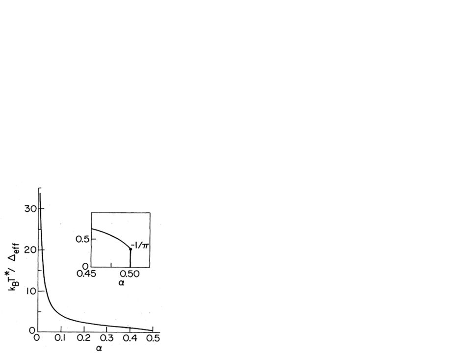
Behaviour depends on  and relative size of parameters:
c

kBTc
Rich, non-trivial dynamics
Cross-over from coherent-incoherent in many ways
All known in terms of experimental parameters
For identical () molecules and c
In particular, at zero temperature and for identical molecules, so epsilon=0, and for Delta << omega_c, the behaviour depends on alpha, the slope of J(omega). For alpha < 1/2, we see coherent oscillations, for alpha between 1/2 and 1 we see incoherent relaxation, and for alpha>1 we see localisation, where the excitation doesn’t move.
What does T=0 mean
Alpha separate
As you’d expect, increasing the temperature destroys both the localisation and coherent
Do up backup slide with more info
Need to explain why goes to zero
Or, rewrite to finite value
Put incoherent graph down to below line
Mention/write that these are graphs of expectation value
Labels on axis (e.g., TIME!!!)
Add <simga_z(t)> to left hand axis
Explain mixed state
16.5
For c, coherent oscillations remain even for high T, 
Bias can help or hinder coherent oscillations

12. Experimental detection of coherent oscillations
Under most “normal” conditions, incoherent transfer
Good for experimentalists using classical theory!
Seeing coherent oscillations:
Identical molecules
Very close
Dipoles unparallel
Selectively excite one with polarised laser pulse
Measure fluorescence anisotropy as excitation moves
Each molecule fluoresces different polarisation - directly monitor z
Highly tunable system (T,c
Change separation, temperature, solvent, genetic engineering
Property
Values 
0-800 meV 
0-100 meV
hc
meV
kBT
meV
Change slide title
Standard(classical)
Include mention of polarisation anisotropy
(reorient molecules in picture?) 19
between

13. Key Results & Conclusions
Demonstrated an experimental realisation of the spin-boson model in terms of coupled biomolecules
Microscopic derivation of the spectral density through minimal models of the surrounding protein and solvent
Dynamics can be observed directly through experiment
Model applicable to other scenarios
Retinal in vision
Photosynthesis
More complex protein models
Molecular biophysics may be a useful testing ground for models of quantum decoherence
Complex but tuneable systems - self assembling too!
It doesn’t always have to be physics helping advance biology! Sometimes, biology can help physics too!
It’s non-trivial to show why FRET is usually incoherent
Can describes

14. Acknowledgements Ross McKenzie (UQ) Paul Meredith (UQ) Ben Powell (UQ)
Andrew Briggs & all at QIPIRC (Oxford)
Gilmore and McKenzie, J. Phys.:Cond. Matt. 17, 1735 (2005)
and quant-ph/ , to appear in Chem. Phys. Lett

15. Quantum mechanics in biology
Classical biology!
Ball and stick models
DNA
No quantum courses for biologists…
Quantum biology!
Highly efficient photosynthesis
Ultrafast vision receptors
Tunneling in enzymes
Quantum consciousness?!
(Okay, probably not)
Exciting = not-boring
1min
Quantum or classical - What decides?

16. A Quantum Vision
Rhodopsin undergoes an ultra-fast, ultra-efficient shape change when it absorbs a photon. How?
Molecule involved in vision
Undergoes ultra-fast and efficient shape change on absorbing light
Only explained by quantum mechanical models
Conical intersections play an important role
The surrounding protein scaffolding
(rhodopsin) is critical for retinal’s function.
Quantum models, involving conical intersections, are necessary.

17. Modelling Need to model many atoms A number of approaches
At very least, choromophore is QM
A number of approaches
Direct QM methods (e.g., DFT)
QM/MM models (some molecules quantum, some not)
We’re trying minimal models
As simple as possible, but no simpler
Capture essential physics, but quick to solve
Very valuable in condensed matter (e.g., Kondo effect)

18. Model for chromophore and its environment
Chromophore properties
Two state system
Point dipole
Protein properties
Spherical, radius b
Continuous medium
Dielectric constant p
Finally, we need the terms which describe the environment. What we’ve done is to consider a minimal model for the interaction between the chromophore and its environment. Towit, we treat the chromophore as a point dipole, which sits inside a uniform, spherical dielectric which represents the protein. And while we’ve thrown away a lot of detail here, generally its electrostatic interactions that dominate the protein’s effects.
Finally, around all this we put the solvent, again represented by a dielectric medium.
Solvent properties
Dielectric constant s()

19. Model for chromophore and its environment
Important physics
Water is strongly polar
Dipole causes polarised solvent “cage”
Reaction field affects dipole
Dynamics
Solvent is fluctuating
Dielectric relaxation, 8ps
Chromophore dipole is different in excited state
The important physics here is that water is strongly polar, and so the point dipole of the chromophore will polarise the solvent (and protein too) surrounding it, forming this “cage” of solvent molecules. In turn, these aligned dipoles will create an electric field, the “reaction field” which acts back on the dipole, stabilising the whole picture. In fact, it’s this interaction which explains why anything dissolves at all.
Very importantly, however, this system isn’t static - the solvent is fluctuating, with its dipole relaxation time of about 8 picoseconds. Further, the magnitude of the chromophore dipole is different in the ground and excited states, meaning that default configuration of the environment changes when the chromophore is excited.
Using this model, we were able to quantise this reaction field, and apply the fluctuation-dissipation relationship to explicitly show that the spin-boson model was appropriate, and derive the spectral density.