Download presentation
Presentation is loading. Please wait.

1
Anisotropic and isotropic electroconvection Collaborators: L.Kramer, W.Pesch (Univ. Bayreuth/Germany and N.Eber (Inst. Solid State Phys./Hungary) OR (low f) NR (high f) I. (anis.)III. (isotr.)II. (interm.) ++ x y H planarhomeotropic
 OR (low f) NR (high f) I. (anis.)III. (isotr.)II. (interm.) ++ x y H planarhomeotropic.")
2
ELECTROHYDRODYNAMICS OF NEMATICS - free energy density - balance of torques - equation of motion - incompressibility - equation of electrostatics -charge conservation STANDARDSTANDARD MODELMODEL (SM)
")
3
Material parameters: Boundary conditions: planar or homeotropic Relevant: alignment + sign of a and a 8 combinations I.planar, a 0 anisotropic II.homeotropic, a 0 intermediate III.homeotropic, a > 0, a < 0 isotropic IV. planar, a < 0, a < 0 non-standard SM

4
I. planar, a 0 anisotropic MBBA: - 0.13 Ginzburg-Landau description works

5
At threshold, increasing f ( planar, a > 0, a < 0 ): ORNR TW (non-stand.) DR n
: ORNR TW (non-stand.) DR n")
6
II. homeotropic, a 0

7
NR OR H drives between semi-isotropic and anisotropic - soft patterning mode - direct transition to STC - AR-s - chevron formation - defect glide - 2 LP-s

8
Homeotropic alignment (standard, semi-isotropic) (A.Rossberg, L.Kramer) theor.exp. OR NR
 (A.Rossberg, L.Kramer) theor.exp. OR NR")
9
III. Homeotropic, a > 0, a < 0 ( truly isotropic) Direct transition to isotropic EC
 Direct transition to isotropic EC")
10
Direct transition to EC -> SM

11
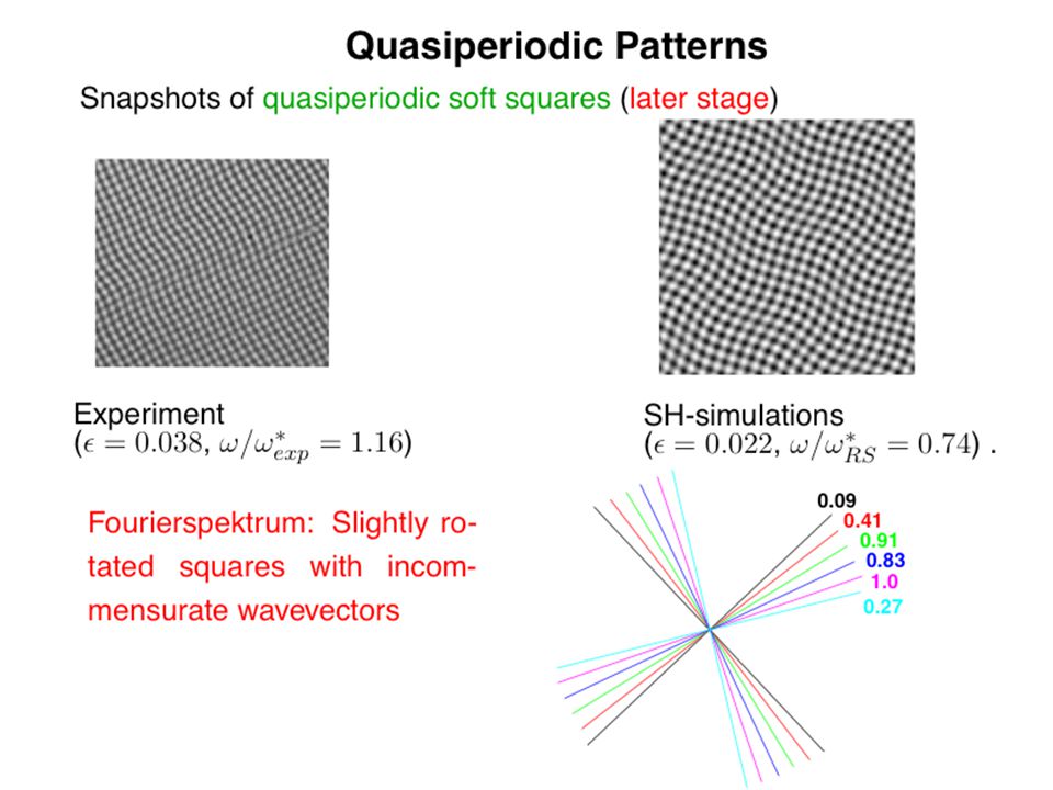
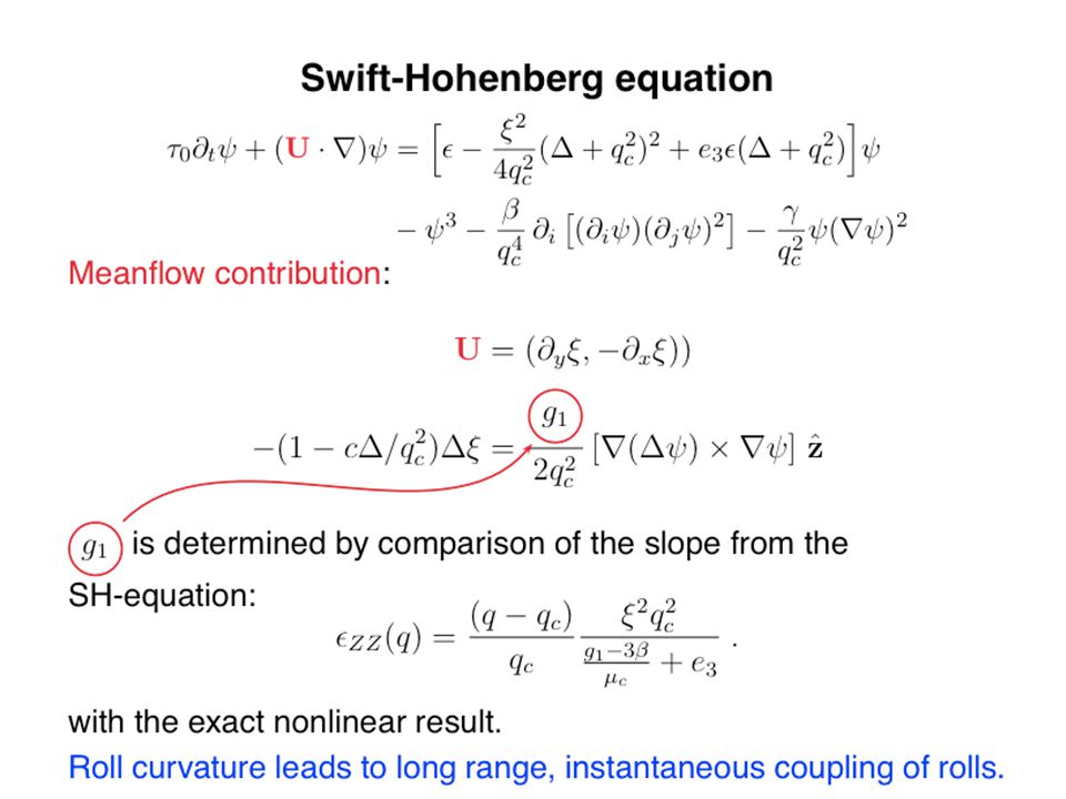
nonlinear regime: hard squares : exp. theo. f At onset: Swift-Hohenberg eq. (W.Pesch, L.Kramer, B.Dressel) soft squares not reproduced
 soft squares not reproduced.")
15
IV. planar, a < 0, a < 0: no standard pattern (conductive)
")
16
- PR or oblique - n z = 0, no shadowgraph - n y (?) oscillates - U c ~ d, f - q c is d indep. Experimental: Dielectric mode! (LK)
.")
17
I and II- conductive III and IV - dielectric

18
1. Dielectric mode for MBBA (planar, a 0) 2. Dielectric mode for MBBA (planar, a < 0, a < 0) - no pattern Flexoelectricity
 - no pattern Flexoelectricity.")
19
Effect on the roll angle, only for d.c. (only in conductive)
")
20
3. Dielectric mode for MBBA (planar, a < 0, a < 0) + flexoelectricity finite threshold! obliqueness! e 1 - e 3 = 1.34 e 1 + e 3 = -7.84

21
4. Dielectric mode for MBBA (planar, a < 0, a < 0) + flexoelectricity e 1 - e 3 = 2.68 e 1 + e 3 = -7.84 (A.Krekhov, W.Pesch)
 + flexoelectricity e 1 - e 3 = 2.68 e 1 + e 3 = (A.Krekhov, W.Pesch).")
22
- dielectric mode at low f - SM + flexoelectricity - why is DM more sensitive to flexo, than CM? planar, a < 0, a < 0: no standard pattern (conductive)
.")
Similar presentations


 3x + 7 = 32 - 2x (ii) 3x + 1 = 5x – 13 (iii) 3(5x – 2) = 4(3x + 6) (iv) 3(2x + 1) = 2x + 11 (v) 2(x + 2)>")


 If >")


 acting on a metal. Take the case when the wavelength of the field is large compared to the electron mean.>")