2. Learning Causality Some slides are from Judea Pearl’s class lecture http://bayes.cs.ucla.edu/BOOK-2K/viewgraphs.html

3. A causal model Example Statement ‘rain causes mud’ implies an asymmetric relationship: the rain will create mud, but the mud will not create rain. Use ‘→’ when refer such causal relationship; There is no arrow between ‘rain’ and ‘other causes of mud’ means that there is no direct causal relationship between them; Rain Other causes of mudMud

4. Directed (causal) Graphs A and B are causally independent; C, D, E, and F are causally dependent on A and B; A and B are direct causes C; A and B are indirect causes D, E and F; If C is prevented from changing with A and B, then A and B will no longer cause changes in D, E and F. A F D E B C

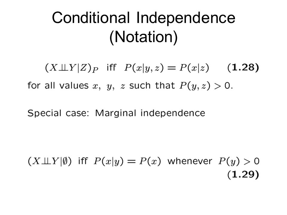
5. Conditional Independence

7. Conditional Independence (Notation)

8. Causal Structure

9. Causal Structure (cont’d) A Causal Structure serves as a blueprint for forming a “casual model” – a precise specification of how each variable is influenced by its parents in the DAG. We assume that Nature is at liberty to impose arbitrary functional relationships between each effect and its causes and then to perturb these relationships by introducing arbitrary disturbance; These disturbances reflect “hidden” or unmeasurable conditions.

10. Causal Model

11. Causal Model (Cont’d) Once a causal model M is formed, it defines a joint probability distribution P(M) over the variables in the system; This distribution reflects some features of the causal structure –Each variable must be independent of its grandparents, given the values of its parents We may allowed to inspect a select subset O  V of “observed” variables to ask questions about P[o], the probability distribution over the observations; We may recover the topology D of the DAG, from features of the probability distribution P[o].

12. Inferred Causation

13. Latent Structure

14. Structure Preference

15. Structure Preference (Cont’d) The set of independencies entailed by a causal structure imposes limits on its power to mimic other structure; L1 cannot be preferred to L2 if there is even one observable dependency that is permitted by L1 and forbidden by L2; L1 is preferred to L2 if L2 has subset of L1’s independence; Thus, test for preference and equivalence can sometimes be reduced to test dependencies, which can be determined by topology of the DAGs without concerning parameters.

16. Minimality

17. Consistency

18. Inferred Causation

19. Examples {a,b,c,d} reveal two independencies: 1.a is independent of b; 2.d is independent of {a,b} given c; Assume further that the data reveals no other independencies; a = having a cold; b = having hay fever; c = having to sneeze; d = having to wipe one’s nose.

20. Example (Cont’d) {a,b,c,d} reveal two independencies: 1.a is independent of b; 2.d is independent of {a,b} given c; minimal Arbitrary relations between a and b Not minimal: fails to impose conditional Independence between d and {a,b} Not consistent with data: impose marginal independence between d and {a,b}

21. Stability The stability condition states that, as we vary the parmeters from  to , no indpendence in P can be destroyed. In other words, if the independency exists, it will always exists.

22. Stable distribution A probability distribution P is a faithful/stable distribution if there exist a directed acyclic graph (DAG) D such that the conditional independence relationship in P is also shown in the D, and vice versa.

23. IC algorithm (Inductive Causation) IC algorithm (Pearl) –Based on variable dependencies; –Find all pairs of variables that are dependent of each other (applying standard statistical method on the database); –Eliminate (as much as possible) indirect dependencies; –Determine directions of dependencies;

24. Comparing abduction, deduction and induction Deduction: major premise: All balls in the box are black minor premise: These balls are from the box conclusion: These balls are black Abduction: rule: All balls in the box are black observation: These balls are black explanation: These balls are from the box Induction: case: These balls are from the box observation: These balls are black hypothesized rule: All ball in the box are black A => B A --------- B A => B B ------------- Possibly A Whenever A then B but not vice versa ------------- Possibly A => B Induction: from specific cases to general rules; Abduction and deduction: both from part of a specific case to other part of the case using general rules (in different ways) Source from httpwww.csee.umbc.edu/~ypeng/F02671/lecture-notes/Ch15.ppt

25. IC Algorithm (Cont’d) Input: –P – a stable distribution on a set V of variables; Output: –A pattern H(P) compatible with P; Patten: is a partially directed DAG some edges are directed and some edges are undirected;

26. IC Algorithm: Step 1 For each pair of variables a and b in V, search for a set S ab such that (a╨b | S ab ) holds in P – in other words, a and b should be independent in P, conditioned on S ab. Construct an undirected graph G such that vertices a and b are connected with an edge if and only if no set S ab can be found. S ab a Not  S ab b  S ab ab ab ╨

27. IC Algorithm: Step 2 For each pair of nonadjacent variables a and b with a common neighbor c, check if c  S ab. If it is, then continue; Else add arrowheads at c i.e a→ c ← b Yes c a b abC ╨ No c a b

28. Example Rain Other causes of mud Mud Rain Other causes of mud Mud

29. IC Algorithm Step 3 In the partially directed graph that results, orient as many of the undirected edges as possible subject to two conditions: –The orientation should not create a new v- structure; –The orientation should not create a directed cycle;

30. Rules required to obtaining a maximally oriented pattern R1: Orient b — c into b→c whenever there is an arrow a→b such that a and c are non adjacent; cbcb bac

31. Rules required to obtaining a maximally oriented pattern R2: Orient a — b into a→b whenever there is a chain a→c→b; baba cab

32. Rules required to obtaining a maximally oriented pattern R3: Orient a — b into a→b whenever there are two chains a — c→b and a — d→b such that c and d are nonadjacent; baba c ab d

33. Rules required to obtaining a maximally oriented pattern R4: Orient a — b into a→b whenever there are two chains a — c→d and c→d→b such that c and b are nonadjacent; baba cad dcb

34. IC* Algorithm Input: –P, a sampled distribution; Output: –core(P), a marked pattern;

35. Marked Pattern:Four types of edges

36. IC* Algorithm: Step 1 For each pair of variables a and b, search for a set S ab such that a and b are independent in P, conditioned on S ab. If there is no such S ab, place an undirected link between the two variables, a – b.

37. IC* Algorithm: Step 2 For each pair of nonadjacent variables a and b with a common neighbor c, check if c  S ab –If it is, then continue; –If it is not, then add arrow heads pointing at c (i.e. a  c  b). In the partially directed graph that results, add (recursively) as many arrowheads as possible, and mark as many edges as possible, according to the following two rules:

38. IC* Algorithm: Rule 1 R1: For each pair of non-adjacent nodes a and b with a common neighbor c, if the link between a and c has an arrow head into c and if the link between c and b has no arrowhead into c, then add an arrow head on the link between c and b pointing at b and mark that link to obtain c –*  b; c a b c a b *

39. IC* Algorithm: Rule 2 R2: If a and b are adjacent and there is a directed path (composed strictly of marked links) from a to b, then add an arrowhead pointing toward b on the link between a and b;