1. Differentiation-Discrete Functions
Mechanical Engineering Majors
Authors: Autar Kaw, Sri Harsha Garapati
Transforming Numerical Methods Education for STEM Undergraduates
4/16/2017

2. Differentiation – ContinuousDiscrete Functions http://numericalmethods

3. Forward Difference Approximation
For a finite

4. Graphical Representation Of Forward Difference Approximation
Figure 1 Graphical Representation of forward difference approximation of first derivative.

5. Example 1
To find contraction of a steel cylinder immersed in a bath of liquid nitrogen, one needs to know the thermal expansion coefficient data as a function of temperature. This data is given for steel in Table 1.
Is the rate of change of coefficient of thermal expansion with respect to temperature more at than at ?
The data given in Table 1 can be regressed to to get Compare the results with part (a) if you used the regression curve to find the rate of change of the coefficient of thermal expansion with respect to temperature at and at

6. Example 1 Cont.
Table 1 Coefficient of thermal expansion as a function of temperature.
Temperature, T
(oF)
Coefficient of thermal expansion,
α (in/in/oF) 80
6.47 40
6.24
−40
5.72
−120
5.09
−200
4.30
−280
3.33
−340
2.45

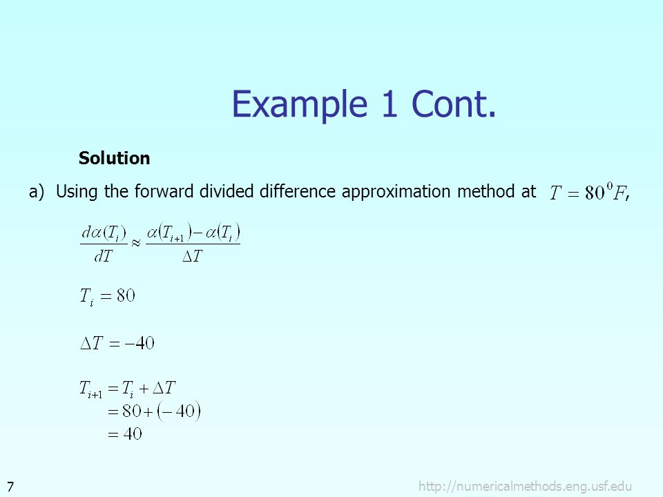
7. Example 1 Cont.
Solution
a) Using the forward divided difference approximation method at ,

8. Example 1 Cont.
Using backwards divided difference approximation method at ,

9. Example 1 Cont.
From the above two results it is clear that the rate of change of coefficient of thermal expansion is more at than at
b) Given

10. Example 1 Cont.
Table 2 Summary of change in coefficient of thermal expansion using
different approximations.
Temperature,
Change in Coefficient of Thermal Expansion,
Divided Difference Approximation
2nd Order Polynomial Regression

11. Direct Fit Polynomials
In this method, given
data points
one can fit a
order polynomial given by
To find the first derivative,
Similarly other derivatives can be found.

12. Example 2-Direct Fit Polynomials
To find contraction of a steel cylinder immersed in a bath of liquid nitrogen, one needs to know the thermal expansion coefficient data as a function of temperature. This data is given for steel in Table 3.
Using the third order polynomial interpolant, find the change in coefficient of thermal expansion at and
The data given in Table 3 can be regressed to to get Compare the results with part (a) if you used the regression curve to find the rate of change of the coefficient of thermal expansion with respect to temperature at and

13. Example 2 Cont.
Table 3 Coefficient of thermal expansion as a function of temperature.
Temperature, T
(oF)
Coefficient of thermal expansion,
α (in/in/oF) 80
6.47 40
6.24
−40
5.72
−120
5.09
−200
4.30
−280
3.33
−340
2.45

14. Example 2-Direct Fit Polynomials cont.
Solution
For the third order polynomial interpolation (also called cubic interpolation), we choose the coefficient of thermal expansion given by
Change in Thermal Expansion Coefficient at :
Since we want to find the rate of change in the thermal expansion coefficient at , and we are using a third order polynomial, we need to choose the four points closest to that also bracket to evaluate it.
The four points are

15. Example 2-Direct Fit Polynomials cont.
such that
Writing the four equations in matrix form, we have

16. Example 2-Direct Fit Polynomials cont.
Solving the above four equations gives
Hence

17. Example 2-Direct Fit Polynomials cont.
Figure 2 Graph of coefficient of thermal expansion vs. temperature.

18. Example 2-Direct Fit Polynomials cont.
The change in coefficient of thermal expansion at is given by
Given that

19. Example 2-Direct Fit Polynomials cont.
b) Change in Thermal Expansion Coefficient at :
Since we want to find the rate of change in the thermal expansion coefficient at , and we are using a third order polynomial, we need to choose the four points closest to that also bracket to evaluate it.
The four points are

20. Example 2-Direct Fit Polynomials cont.
Such that
Writing the four equations in matrix form, we have

21. Example 2-Direct Fit Polynomials cont.
Solving the above four equations gives
Hence

22. Example 2-Direct Fit Polynomials cont.
Figure 3 Graph of coefficient of thermal expansion vs. temperature.

23. Example 2-Direct Fit Polynomials cont.
The change in coefficient of thermal expansion at is given by
Given that

24. Example 2-Direct Fit Polynomials cont.
Table 4 Summary of change in coefficient of thermal expansion using different approximations.
Temperature,
Change in Coefficient of Thermal Expansion,
3rd Order Interpolation
2nd Order Polynomial Regression

25. Lagrange Polynomial In this method, given , one can fit a given by
order Lagrangian polynomial
given by
where ‘
’ in
stands for the
order polynomial that approximates the function
given at
data points as
, and
a weighting function that includes a product of
terms with terms of
omitted.

26. Lagrange Polynomial Cont.
Then to find the first derivative, one can differentiate
once, and so on
for other derivatives.
For example, the second order Lagrange polynomial passing through is
Differentiating equation (2) gives

27. Lagrange Polynomial Cont.
Differentiating again would give the second derivative as

28. Example 3
To find contraction of a steel cylinder immersed in a bath of liquid nitrogen, one needs to know the thermal expansion coefficient data as a function of temperature. This data is given for steel in Table 5.
Using the second order Lagrange polynomial interpolant, find the change in coefficient of thermal expansion at and
The data given in Table 5 can be regressed to to get Compare the results with part (a) if you used the regression curve to find the rate of change of the coefficient of thermal expansion with respect to temperature at and

29. Example 3 Cont.
Table 5 Coefficient of thermal expansion as a function of temperature.
Temperature, T
(oF)
Coefficient of thermal expansion,
α (in/in/oF) 80
6.47 40
6.24
−40
5.72
−120
5.09
−200
4.30
−280
3.33
−340
2.45

30. Example 3 Cont.
Solution
For second order Lagrangian interpolation, we choose the coefficient of thermal expansion given by
Change in the thermal expansion coefficient at :
Since we want to find the rate of change in the thermal expansion coefficient at and we are using second order Lagrangian interpolation, we need to choose the three points closest to that also bracket to evaluate it.
The three points are

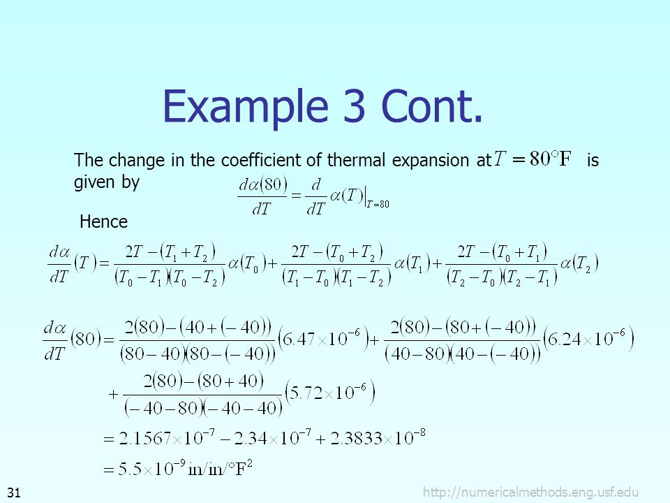
31. Example 3 Cont.
The change in the coefficient of thermal expansion at is given by
Hence

32. Example 3 Cont. b) Change in the thermal expansion coefficient at :
Since we want to find the rate of change in the thermal expansion coefficient at and we are using second order Lagrangian interpolation, we need to choose the three points closest to that also bracket to evaluate it.
The three points are
The change in the coefficient of thermal expansion at is given by

33. Example 3 Cont.
Hence

34. Example 3 Cont.
Table 6 Summary of change in coefficient of thermal expansion using different approximations.
Temperature,
Change in Coefficient of Thermal Expansion,
2nd Order Lagrange Interpolation
2nd Order Polynomial Regression

35. Additional Resources
For all resources on this topic such as digital audiovisual lectures, primers, textbook chapters, multiple-choice tests, worksheets in MATLAB, MATHEMATICA, MathCad and MAPLE, blogs, related physical problems, please visit

36. THE END