1. Adiabaticity in Open Quantum Systems: Geometric Phases & Adiabatic Quantum Computing Joint work with Dr. Marcelo Sarandy Adiabatic Approximation in Open Quantum Systems, Phys. Rev. A 71, 012331 (2005) Adiabatic Quantum Computation in Open Systems, Phys. Rev. Lett. 95, 250503 (2005) Geometric Phases in Adiabatic Open Quantum Systems, quant-ph/0507012 (submitted) [Holonomic Quantum Computation in Decoherence-Free Subspaces, Phys. Rev. Lett. 95, 130501 (2005)] $: USC Center for Quantum Information Science and Technology CQIST

2. Adiabatic Theorem If Hamiltonian “changes slowly” then “no transitions”, i.e.: Energy eigenspaces evolve continuously and do not cross. Applications abound… Standard formulation of adiabatic theorem: applies to closed quantum systems only (Born & Fock (1928); Kato (1950); Messiah (1962)). This talk: - A generalization of the adiabatic approximation to the case of open quantum systems. - Applications to adiabatic quantum computing & geometric phases. - We’ll show (main result): adiabatic approximation generically breaks down after long enough evolution. The Adiabatic Approximation

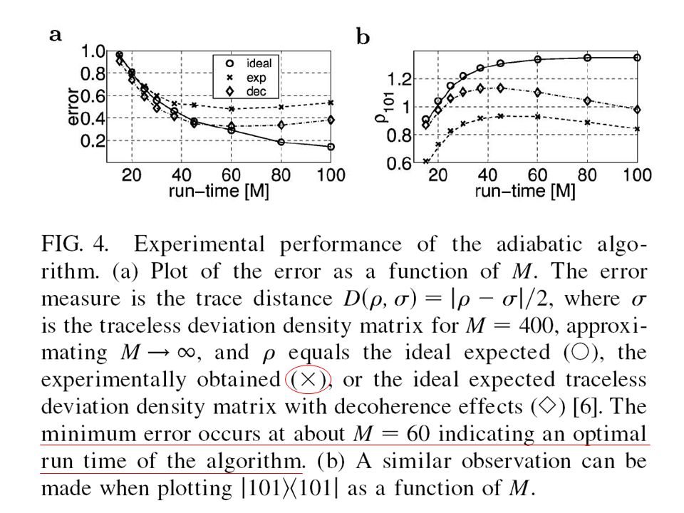
3. Experimental Evidence for Finite-Time Adiabaticity in an Open System

5. Intuition for optimal time: Decoherence causes broadening of system energy levels (many bath levels accessible), until they overlap. Competition between adiabatic time (slow) and need to avoid decoherence (fast) yields optimal run time.

6. Open Quantum Systems systembath Every real-life quantum system is coupled to an environment (“bath”). Full Hamiltonian: Environment (Bath) System Open quantum systems are not described by the Schrodinger equation Common textbook statement: “We’ve never observed a violation of the Schrodinger equation”

7. Reduced Description Recipe for reduced description of system only = trace out the bath: Exact (Kraus Representation) – full account of bath memory:

8. After certain approximations (e.g. weak-coupling) can obtain general class of (generally non-Markovian) master equations. Convolutionless master equation: Master Equations

9. Spectrum via the Jordan block-diagonal form PRA 71, 012331 (2005)

10. Left and Right Eigenvectors PRA 71, 012331 (2005) Jordan block index row index inside given Jordan block J J J

11. Definition of Adiabaticity in closed/open systems Adiabaticity in open quantum systems: An open quantum system is said to undergo adiabatic dynamics if its evolution is so slow that it proceeds independently in sets of decoupled superoperator-Jordan blocks associated to distinct eigenvalues of L (t). Adiabaticity in closed quantum systems: A closed quantum system is said to undergo adiabatic dynamics if its evolution is so slow that it proceeds independently in decoupled Hamiltonian-eigenspaces associated to distinct eigenvalues of H (t). Note: Definitions agree in closed-system limit of open systems, since L (t) becomes the Hamiltonian superoperator [H,.]. PRA 71, 012331 (2005)

12. Simple “Derivation” of Adiabaticity – closed systems Time-dependent Schrodinger equation: Instantaneous diagonalization: Together yield: X system state in basis of eigenvectors of H(t). since H d (t) is diagonal, system evolves separately in each energy sector. = the adiabatic approximation. PRA 71, 012331 (2005)

13. Simple “Derivation” of Adiabaticity – open systems Time-dependent master equation: Instantaneous Jordanization: Together yield: X system state in basis of right eigenvectors of L (t). = the adiabatic approximation. PRA 71, 012331 (2005)

14. Closed system adiabatic dynamics takes place in decoupled eigenspaces of time-dependent Hamiltonian H PRA 71, 012331 (2005) adiabatic eigenspaces

15. Open system adiabatic dynamics takes place in decoupled Jordan-blocks of dynamical superoperator L adiabatic blocks PRA 71, 012331 (2005)

16. Remark on Order of Operations PRA 71, 012331 (2005) We chose 3. since 1. System and bath generally subject to different time scales. May also be impractical. 2. Adiabatic limit on system is not well defined when bath degrees of freedom are still explicitly present.

17. Time Condition for Adiabatic Dynamics Condition for adiabaticity: Total evolution time can be lower-bounded by max. norm of time-derivative of generator (H or L ) min. square of |spectral gap| (energies or complex-valued Jordan eigenvalues) What is the analogous condition for open systems? ) ) PRA 71, 012331 (2005) power

18. 1D Jordan blocks Time Condition for Open Systems Adiabaticity numerical factor time-derivate of generator spectral gap Remarks: The crossover time provides a decoupling timescale for each Jordan block If there is a growing exponential ( real and positive) then adiabaticity persists over a finite time interval, then disappears! This implies existence of optimal time for adiabaticity

19. Application 1: Adiabatic Quantum Computing Farhi et al., Science 292, 472 (2001) Measure individual spin states and find answer to hard computational question! Procedure’s success depends on gap not being too small:

20. Adiabatic QC can only be performed while adiabatic approximation is valid. Breakdown of adiabaticity in an open system implies same for AQC. Implications for Adiabatic QC M.S. Sarandy, DAL, Phys. Rev. Lett. 95, 250503 (2005) Robustness of adiabatic QC depends on presence of non-vanishing gap in spectrum. Can we somehow preserve the gap? Yes, using a “unitary interpolation strategy” [see also M.S. Siu, PRA ’05]. We have found: A constant gap is possible in the Markovian weak-coupling limit A constant gap is non-generic in non-Markovian case

21. Unitary Interpolation: Adiabatic Open Systems *Note: constant super-operator spectrum implies constant gaps in Hamiltonian spectrum * C In adiabatic + weak-coupling limit leading to the Markovian master equation, Lindblad operators must follow Hamiltonian (Davies & Spohn, J. Stat. Phys. ’78). But otherwise this condition is non-generic. Phys. Rev. Lett. 95, 250503 (2005)

22. Example: Deutsch-Josza Algorithm under (non-Markovian) Dephasing Phys. Rev. Lett. 95, 250503 (2005)

23. Additional comments: - Gaps constant in spite of non- Markovian model. True also for spontaneous emission in this example. - Four 1D Jordan blocks; one automatically decoupled. Hence adiabaticity depends on decoupling of other three. Phys. Rev. Lett. 95, 250503 (2005)

24. di Phys. Rev. Lett. 95, 250503 (2005)

25. Adiabatic QC can only be performed while adiabatic approximation is valid. However, the adiabatic approximation (typically) breaks down in an open system if the evolution is sufficiently long. Breakdown of adiabaticity in an open system implies same for AQC. Breakdown is due to vanishing of gaps, due to interaction with environment. Gaps can be kept constant via unitary interpolation (at expense of introducing many-body interactions) when bath is Markovian. Error correction techniques a la Jordan, Shor & Farhi are needed. Summary of Conclusions for Adiabatic QC Phys. Rev. Lett. 95, 250503 (2005)

26. Application 2: Geometric Phases Adiabatic cyclic geometric phase: A non-dynamic phase factor acquired by a quantum system undergoing adiabatic evolution driven externally via a cyclic transformation. The phase depends on the geometrical properties of the parameter space of the Hamiltonian. –Berry (Abelian) phase: non-degenerate states –Wilczek-Zee (non-Abelian) phase: degenerate states

27. Open Systems Geometric Phase Substituting: Convolutionless master equation, implicit time-dependence through parameters : Solve by expanding d.m. in right eigenbasis, explicitly factor out dynamical phase Simplification for single, 1D, non-degenerate Jordan block: Solution: Abelian Geometric Phase: quant-ph/0507012

28. Abelian Geometric Phase: quant-ph/0507012

29. Non-Abelian Open Systems Geometric Phase Case of degenerate 1D Jordan blocks: Rewrite:where Wilson loop: Solution: non-Abelian Wilczek-Zee gauge potential; holonomic connection: Geometric, gauge-invariant, correct closed-system limit, complex valued. quant-ph/0507012

30. Berry’s Example: Spin-1/2 in Magnetic Field Under Decoherence System Hamiltonian: In adiabatic + weak-coupling limit leading to the Markovian master equation, Lindblad operators must follow Hamiltonian (Davies & Spohn, J. Stat. Phys. ’78) : Dephasing: Spontaneous emission: diagonalizes Superoperator:, diagonalizable, hence diagonalizable in eigenbasis. But eigenbasis doesn’t depend on Hence geometric phase immune to dephasing and spont. emission! Closed system result reproduced.

31. Adiabaticity time does depend on. I.e., adiabatic geometric phase disappears when adiabatic approximation breaks down. Results for spherically symmetric B-field, azimuthal angle=  /3 too short too long quant-ph/0507012 condition for adiabaticity:

32. Geometric phase is not invariant under bit flip: quant-ph/0507012 geometric phase in units of  Results for spherically symmetric B-field, azimuthal angle=  /3

33. QC: How to deal with non-robustness of geometric phase under decoherence?

34. USC Center for Quantum Information Science and Technology CQIST Summary Adiabaticity defined for open systems in terms of decoupling of Jordan blocks of super-operator Central feature: adiabaticity can be a temporary feature in an open system Implications for robustness of adiabatic QC and for geometric phases in open systems Phys. Rev. A 71, 012331 (2005); Phys. Rev. Lett. 95, 130501 (2005); Phys. Rev. Lett. 95, 250503 (2005); quant-ph/0507012.