1. Lecture 3

2. Summary of Lecture 2 The three types of interactions that optical methods exploit to yield biomedical information about cells and tissues are: –Scattering Elastic scattering (scattered frequency same as incident) –Multiple scattering ----Diffuse reflectance spectroscopy, Diffuse optical tomography –Single scattering ----Light scattering spectroscopy, Microscopy, Optical Coherence Tomography Inelastic scattering (scattered frequency shifted with respect to incident) –Raman spectroscopy –Absorption Radationless relaxation ---- Diffuse reflectance spectroscopy, Diffuse optical tomography –fluorescence To understand the wavelength/energy dependent nature of these processes, we need to understand how light interacts with matter

3. Summary of Lecture 2 The basic unit of matter is the –atom Atoms consist of –a nucleus surrounded by electron(s) It is impossible to know exactly both the location and velocity of a particle at the same time Describe the probability of finding a particle within a given space in terms of a –wave function, 

4. Summary of Lecture 2 The wavefunction of an electron is also called an –orbital We draw orbitals to represent the space within which we have 90% probability of finding an electron To find the wavefunction(s) representing the electronic state(s) of an atom we need to solve –the Schrödinger equation

5. Summary of Lecture 2 The particle confined in a one-dimensional box of length a, represents a simple case, with well-defined wavefunctions and corresponding energy levels n can be any positive integer, 1,2,3…, and represents the number of nodes (places where the wavefunction is zero) Only discrete energy levels are available to the particle in a box----energy is quantized

6. Atomic orbitals: Hydrogen atom The Schrödinger equation can be formulated and solved for a hydrogen atom, consisting of a negatively charged electron moving around a positively charged nucleus (i.e. electron has potential energy due to nuclear attraction, ) R nl describes how wave function varies with distance of electron from nucleus Y lm describes the angular dependence of the wave function Subscripts n, l and m are the quantum numbers of hydrogen

7. Quantum numbers Principal quantum number, n –Has integral values of 1,2,3…… and is related to size and energy of the orbital Angular quantum number, l –Can have values of 0 to n-1 for each value of n and relates to the angular momentum of the electron in an orbital; it defines the shape of the orbital Magnetic quantum number, m l –Can have integral values between l and - l, including zero and relates to the orientation in space of the angular momentum. Electron spin quantum number, m s –This quantum number only has two values: ½ and –½ and relates to spin orientation

8. Rules for filling electronic states Pauli exclusion principle No two electrons can have the same set of quantum numbers: n, l, m l and m s Aufbau principle Electrons fill in the orbitals of successively increasing energy, starting with the lowest energy orbital Hund’s rule For a given shell (example, n=2), the electron occupies each subshell one at a time before pairing up

9. Example: Br (35 electrons) Electronic configuration: 1s 2 2s 2 2p 6 3s 2 3p 6 4s 2 3d 10 4p 5

11. Molecular Orbitals 1.Introduction to molecular orbitals 2.Bonding vs. antibonding orbitals  (sigma) and  (pi) bonds

12. Introduction to molecular orbitals Molecular orbitals (chemical bonds) originate from –the overlap of occupied atomic orbitals Only the valence electrons of atomic orbitals contribute significantly to molecular orbitals –Oxygen 1s 2 2s 2 2p 4 –Has 6 valence electrons –Xenon : 1s 2 2s 2 2p 6 3s 2 3p 6 4s 2 3d 10 4p 6 5s 2 4d 10 5p 6 –has 8 valence electrons Each molecular orbital can hold two electrons; spins must be opposite

13. Bonding vs. anti-bonding orbitals Bonding molecular orbital: lower in energy than the atomic orbitals of which it is made Antibonding molecular orbital: higher in energy than the atomic orbitals of which it is made Antibonding character indicated by asterisk.

14. Molecular orbitals  Bonds Involve s orbitals and p orbitals Overlap of two atomic orbitals along the line joining nuclei of bonded atoms Charge distribution is localized along bond axis Electrons in  bonds are tightly bound; lots of energy required to vacate molecular orbitals

15. Sigma (  ) bonds bonding Anti-bonding

16. Molecular orbitals  Bonds Involves p or d orbitals Overlap of two atomic orbitals at right angles to the line joining the nuclei of bonded atoms Charge distribution is above and below plane containing  bond Less tightly bound

17. Pi (  ) bonds bondingAnti-bonding

18. Bond order=3 Bond order: 3 (# of e- in bonding orb)-(# of e- in anti-bonding orb) 2

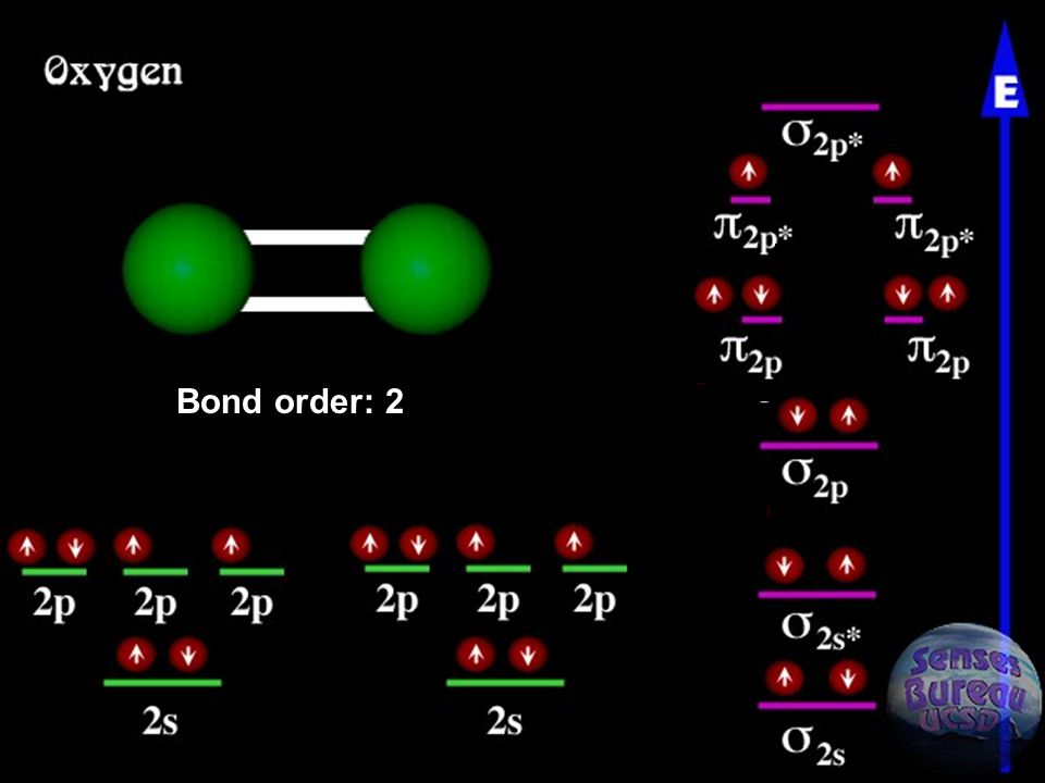
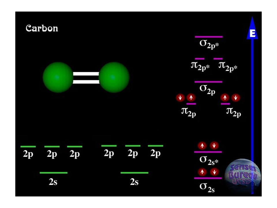
19. Bond order: 2

26. Molecular orbitals Molecular orbitals (chemical bonds) originate from the overlap of occupied atomic orbitals Bonding molecular orbitals –are lower in energy than corresponding atomic orbitals (stabilizes the molecule) Anti-bonding orbitals –are higher in energy than corresponding atomic orbitals and destabilizes the molecule  bonds –involve overlapping s and p orbitals along the line joining the nuclei of the bond-forming atoms  bonds –involve p and d orbitals overlapping above and below the line joining the nuclei of the bond-forming atoms

27. Molecular orbitals Only the valence electrons of atomic orbitals contribute significantly to molecular orbitals –Oxygen has 6 valence electrons: 1s 2 2s 2 2p 4 –Xenon has 8 valence electrons: 1s 2 2s 2 2p 6 3s 2 3p 6 4s 2 3d 10 4p 6 5s 2 4d 10 5p 6 Each molecular orbital can hold two electrons; spins must be opposite Number of available molecular orbitals equals the sum of original atomic orbitals

28. Polyatomic molecules: hybridization Valence bond theory cannot explain the bonding or the structure of polyatomic molecules Carbon, for example, has in its ground state only two unpaired electrons in two 2p orbitals. Thus, carbon should form only two bonds. However, carbon almost always forms four bonds

29. Hybridization: sp 3 orbitals To explain how carbon forms its four bonds, we assume that one of the 2s electrons is “promoted” or “excited” to one of the unoccupied 2p orbitals With the 2s orbital half empty and the 2p orbitals all having electrons with parallel spin, the orbitals merge to form four equal energy orbitals, arranged in a tetrahedral geometry (bond angle-109.5º)

30. Methane: sp 3 orbitals Why sp 3 orbitals? –Each sp 3 orbital has a large lobe, which makes it easier to overlap with another orbital, such as that of a hydrogen atom

31. sp hybrid formation When a 2s and a 2p bond combine they need to form two bonds, equivalent in shape and energy Think of the resulting orbitals as the shapes that arise either when you add the 2s and the 2p orbitals or when you subtract the 2p from the 2s orbital

32. sp hybrid orbitals: triple bonds A carbon atom with 2 sp orbitals still has one electron in each one of the two p bonds What happens when two such atoms form a molecular bond? acetylene

33. sp 2 orbitals: double bonds What happens when a 2s orbital mixes with two 2p orbitals? How many orbitals are formed and at what orientation? Three sp 2 hybrid orbitals form, arranged on a plane at 120 º from each other

34. sp 2 hybrid orbitals: double bonds Does a carbon atom with 3 sp 2 orbitals still have any other electrons? What happens when two such atoms form a molecular bond? One  sp2 bond and one  bond are formed

35. Origin of UV-Visible spectra: conjugated bonds Conjugated organic molecules consist of alternating single and multiple bonds between chains of carbon atoms 1,3-butadiene H 2 C=CH-CH=CH 2 Carbon and hydrogen atoms are bonded so that each carbon atom is left with an unused electron in a 2p orbital, with the 2p bonds parallel to each other

36. Conjugated bonds The four 2p orbitals can combine to form these  orbitals, arranged according to energy, with the lowest energy  orbital at the bottom. Can you think of a set of wavefunctions that may describe what is going on? These are similar to the wavefunctions we got for a particle in the box, with the length of the box corresponding to the length of the carbon chain

37. Conjugated bonds and particle in a box The four 2p orbitals can combine to form these  orbitals, arranged according to energy, with the lowest energy  orbital at the bottom. How will the electrons be distributed? Each of the orbitals can accommodate two electrons. Since there are 4 electrons, the two lower orbitals will be occupied 4 2p AO 11 22 33 44 Highest Filled Orbital Lowest Unfilled Orbital

38. Conjugated bonds and particle in a box What will be the energy required for an electron to be excited from such a bonding to an anti-bonding  orbital? 4 2p AO 11 22 33 44 Highest Filled Orbital Lowest Unfilled Orbital What can provide the energy for this transition? The energy for this transition can be provided by a photon with energy E=hv=hc/

39. Origin of UV-visible spectra For UV-Visible spectroscopy relevant electronic transitions involve n→  and  →  transitions Compound  nm) transition with lowest energy CH4122  * (C-H) CH3CH3130  * (C-C) CH3OH183 n-  * (C-O) CH3SH235 n-  * (C-S) CH3NH2210 n-  * (C-N) CH3Cl173 n-  * (C-Cl) CH3I258 n-  * (C-I) CH2=CH2165  * (C=C) CH3COCH3187  * (C=O) 273 n-  * (C=O) CH3CSCH3460 n-  * (C=S) CH3N=NCH3347 n-  * (N=N)

40. Some chromophores of interest Beta carotene

41. Energy Levels Definition Energy levels are characteristic states of a molecule Ground state is state of lowest energy States of higher energy are called excited states

42. Energy Levels Classification of Energies Can you think of some types of energies associated with a molecule? A molecule can be thought of as having several distinct reservoirs of energy E molecule = E translation ( motion of the molecule’s center of mass through space) + E electron spin (orientation of nuclear spin in a magnetic field) + E nuclear spin (orientation of electron spin in a magnetic field) + E rotation (rotation of the molecule about its center of mass) + E vibration ( vibration of the molecule’s constituent atoms ) + E electronic (electronic transitions between available energy states) The energy associated with each of these are quantized

43. Energy Levels

44. EnergyEnergy Level Separation (J) TranslationVery small Spin10 -32 Rotation10 -28 Vibration10 -25 Electronic10 -19

45. Energy Levels EM spectrum

46. Energy Levels EM Radiation Energy Levels Radio Frequency Spin Orientation MicrowaveRotational IRVibrational U UV- VISElectronic

47. Energy Levels Electronic energy levels Electronic energy levels of molecules are described by molecular orbitals When an electron undergoes an electronic transition, it is transferred from one molecular orbital to another UV-VIS absorption / fluorescence spectroscopy involves electronic energy transitions

48. Energy Levels Atomic energy levels Each energy level in the system corresponds to the potential energy between the positive and negative charges The potential energy results from the force between particles, i.e., the nucleus and electron (Coulombic force) + -e r (radius) +e F

49. Energy Levels Atomic energy levels The electronic energy level is constant for each energy level, when the distance between the electron and nucleus is constant

50. Energy Levels Molecular energy levels How does energy level change with inter-nuclear distance? Example, 1s orbital of Hydrogen. R = 0* R = infinity Sigma bond *chemically unfeasible limit when nuclei fuse together

51. Energy Levels Molecular energy levels Energy of a pair of atoms as a function of distance between them is given by the Morse curve, where R 2 is the equilibrium bond distance Stretching or compressing the bond gives an increase in the energy Morse curve can be approximated by a simple Hooke’s law function V=.5*k(R-R 2 ) 2 +.5*k’(R-R 2 ) 3 +.5*k’’(R-R 2 ) 4