Download presentation
Presentation is loading. Please wait.

2
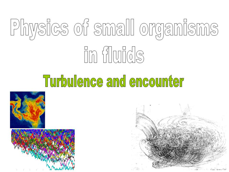
Turbulence: an intuitive understanding

3
Found in all fluids at a variety of scales Soap bubble Circulation in the atmosphere of Jupiter Magnetically stirred fluid in the lab Coccolithophore bloom in the North Sea

4
Mechanical Energy In Mechanical Energy Out Turbulence Heat large scale small scale Cascade of inertia (mechanical energy)
")
5
Andrei Kolmogorov Energy cascade Conserve angular momentum ( ) and kinetic energy (1/2 u 2 ) =L =L/2....... Kolmogorov spectra theory

6
wave number, k (2 /ℓ) energy density spectrum, E(k) (L 3 /T 2 ) Governed by 2 parameters viscosity dissipation rate Kolmogorov spectra theory
 energy density spectrum, E(k) (L 3 /T 2 ) Governed by 2 parameters viscosity dissipation rate Kolmogorov spectra theory")
7
kk Kolmogorov spectra measured in nature

8
Turbulent dissipation rate is becoming a routine physical measurement m 2 /s 3 = W/kg Microstructure Shear Probe Sinks freely through the water column Measuring turbulence in nature

9
Yamazaki et al 2002 The Sea v 12 Dissiption rate varies vertically Measuring turbulence in nature

10
Visser et al, Mar Biol 2001 Dissiption rate varies in time Measuring turbulence in nature

11
>10 -3 m 2 /s 3 tidal currents <10 -10 m 2 /s 3 deep ocean 10 -8 m 2 /s 3 themocline 10 -6 to 10 -4 m 2 /s 3 surface Typical values of dissipation rate units: m 3 /s 3 = W/kg = 10 4 cm 2 /s 3 wind surface waves bottom friction internal waves damping in thermocline Vertical structure Measuring turbulence in nature

12
Oliver Ross, Thesis, SOC 2002 turbulence closure schemes Tidal currents Modelling turbulence in nature

13
Turbulent dispersion How 2 particles move relative to each other what are the statistics of the variance of the interparticle separation could be molecules could be organisms scale dependent For a diffusive process 2 = 2 D t

14
02-2-4-6-846 log 10 Scale (m) Molecular diffusion vertical horizontal Turbulent eddy diffusion Richardson’s law Kolmogorov scaleIntegral length scaleBatchelor scale Turbulent straining phytoplankton hetertrophic protists adult copeods larval fish Turbulent dispersion
 Molecular diffusion vertical horizontal Turbulent eddy diffusion Richardson’s law Kolmogorov scaleIntegral length scaleBatchelor scale Turbulent straining phytoplankton hetertrophic protists adult copeods larval fish Turbulent dispersion")
15
D (cm 2 /s) 10m1km100km ℓ 4/3 ℓ 11 22 nn NN x0x0 Diffusivity = the time rate of change of Scale dependent Turbulent dispersion: Richardsons law (inertial subrange)
 10m1km100km ℓ 4/3 ℓ 11 22 nn NN x0x0 Diffusivity = the time rate of change of Scale dependent Turbulent dispersion: Richardsons law (inertial subrange)")
16
Relative motion and turbulence Turbulence increases the relative motion of particles Richardson's law for scales within the inertial subrange also for scales within the viscous subrange w( ) = ( ) 1/3 w( ) = = ( / ) 1/2
 = ( ) 1/3 w( ) = = ( / ) 1/2 ")
17
The stucture function Separation distance (units of Kolmogorov scale) 0.1110100 Velocity difference (arbitrary scale) 0.1 1 10 Kolmogorov scale Inertia dominates velocity difference ~ 1/3 Viscosity dominates velocity difference ~ Relative motion and turbulence In nature 1 to 0.1 cm
 Velocity difference (arbitrary scale) Kolmogorov scale Inertia dominates velocity difference ~ 1/3 Viscosity dominates velocity difference ~ Relative motion and turbulence In nature 1 to 0.1 cm")
18
Encounter rate and turbulence (1) The Up Side u v R w Rothschild & Osborn, J Plankton Res 1988 Evans, J Plankton Res 1989 Visser & MacKenzie, J Plankton Res 1998 w = ( R) 1/3 Z = C = C R 2 (u 2 + v 2 + 2w 2 ) 1/2 is the encounter kernel ≈ maximum clearance rate turbulent velocity scale prey predator perception distance
 The Up Side u v R w Rothschild & Osborn, J Plankton Res 1988 Evans, J Plankton Res 1989 Visser & MacKenzie, J Plankton Res 1998 w = ( R) 1/3 Z = C = C R 2 (u 2 + v 2 + 2w 2 ) 1/2 is the encounter kernel ≈ maximum clearance rate turbulent velocity scale prey predator perception distance")
19
Encounter rate and turbulence (1) The Up Side Encounter rate turbulent dissipation rate component due solely to behaviour increase due to turbulence
 The Up Side Encounter rate turbulent dissipation rate component due solely to behaviour increase due to turbulence")
20
Encounter rate and turbulence (2) Ingestion rate Encounter rate is not the same as ingestion rate Functional response is handling time turbulent dissipation rate Ingestion rate concentration increases -1
 Ingestion rate Encounter rate is not the same as ingestion rate Functional response is handling time turbulent dissipation rate Ingestion rate concentration increases -1")
21
Acartia tonsa feeding on ciliates Dissipation rate, cm 2 s 10 -7 10 -6 10 -5 10 -4 10 -3 10 -2 10 10 0 1 2 Clearance rate, cm3 / day 0 200 400 600 800 1000 Observed Predicted what happens here ? Encounter rate and turbulence from the lab

22
Encounter rate and turbulence (3) The Down Side Turbulence interferes with the remote detection ability of organisms hydromechanical chemical Turbulence sweeps prey out of the detection zone before organísms can capture them Turbulence interferes with the structure and efficiency of feeding currents
 The Down Side Turbulence interferes with the remote detection ability of organisms hydromechanical chemical Turbulence sweeps prey out of the detection zone before organísms can capture them Turbulence interferes with the structure and efficiency of feeding currents")
23
Saiz, Calbet & Broglio Limnol Oceanogr 2003 Encounter rate and turbulence from the lab

24
Visser, Saito, Saiz & Kiørboe, Mar Biol (2001) Calanus finmarchicus Some species appear to be impeded by turbulence Encounter rate and turbulence from the field October 1998 16171819202122232425 Filtering index, f 0 5 10 15 20 f = gut content/ambient chl
 Calanus finmarchicus Some species appear to be impeded by turbulence Encounter rate and turbulence from the field October Filtering index, f f = gut content/ambient chl")
25
Visser, Saito, Saiz & Kiørboe, Mar Biol (2001) Oithona similis Encounter rate and turbulence from the field Some species appear to migrate vertically to mitigate the effects of strong turbulence
 Oithona similis Encounter rate and turbulence from the field Some species appear to migrate vertically to mitigate the effects of strong turbulence")
26
Reaction (detection) distance is a function of: Predator size b and sensitivity s Prey size a, velocity u and mode of motion Turbulence vrs signal strength u v w a Encounter rate and turbulence: Factors effecting detection
 distance is a function of: Predator size b and sensitivity s Prey size a, velocity u and mode of motion Turbulence vrs signal strength u v w a Encounter rate and turbulence: Factors effecting detection")
27
Signal to noise ratio Reaction (detection) distance in turbulent waters r velocity U radius a 2b2b Self-propelled body at low Reynolds number u(r) = U(a/r) 2 Reaction (detection) distance in still water Visser, Mar Ecol Prog Ser 2001 R 0 a(U/s) 1/2 Encounter rate and turbulence: Signal to noise
 distance in turbulent waters r velocity U radius a 2b2b Self-propelled body at low Reynolds number u(r) = U(a/r) 2 Reaction (detection) distance in still water Visser, Mar Ecol Prog Ser 2001 R 0 a(U/s) 1/2 Encounter rate and turbulence: Signal to noise")
28
-3-2012 -1.7 -1.6 -1.5 -1.4 -1.3 -1.2 -1.1 -0.9 Log 10 ( ) Log 10 (R) Laboratory study of Acartia tonsa feeding on ciliate Strombidium sulcatum under turbulent conditions Saiz E, Kiørboe T, 1995. Mar Ecol Prog Ser observed clearence rate o and solving o = R 2 (v 2 + 2 2 ( R) 2/3 ) 1/2 agitation rateCoefficients: intercept = 1.343 slope = 0.167 r² = 0.965 R 1/6 Detection distance dependence on turbulent dissipation rate
 2/3 ) 1/2 agitation rateCoefficients: intercept = slope = r² = R 1/6 Detection distance dependence on turbulent dissipation rate.")
29
Increased ingestion rate due to more encounters Decreased ingestion rate due to impaired detection – caputre efficiency turbulence Ingestion rate Dome – shaped response Active avoidance of high turbulence zones Change of feeding mode with turbulence Behavioural shifts Interaction specific Encounter rate and turbulence: Dome - shape

30
znzn z n+1 = r (2 D) 1/2 r is a random number such that mean(r) = 0 variance(r) = 1 is the time step between evaluations D is the diffusivity Modelling turbulent diffusion: random walk how much light a phytoplankton cell receives depth
 1/2 r is a random number such that mean(r) = 0 variance(r) = 1 is the time step between evaluations D is the diffusivity Modelling turbulent diffusion: random walk how much light a phytoplankton cell receives depth")
31
Depth(m) Time(hours) Modelling turbulent diffusion: random walk
 Time(hours) Modelling turbulent diffusion: random walk")
32
Depth(m) Time(hours) Modelling turbulent diffusion: random walk
 Time(hours) Modelling turbulent diffusion: random walk")
33
Visser 1997 diffusivitydistribution depth Unmixes an initially uniform distribution vertical random walk distribution predicted by Modelling turbulent diffusion: what can go wrong

34
diffusivitydistribution depth vertical random walk vertically uniform distribution as predicted by diffusion equn. Modelling turbulent diffusion: corrected for accumulation Visser 1997

35
time Length of filament ~ exp( t) Variance 2 ~ t to t 3 Turbulence and distribution patterns A blob of ink in a stirred fluid
 Variance 2 ~ t to t 3 Turbulence and distribution patterns A blob of ink in a stirred fluid")
36
Plankton distribution Distribution of solutes Photo: Alice Alldredge 100’s km 100’s µm Turbulence and distribution patterns Diffusion is useful in describing the probability of a distribution BUT Any given distribution does not look diffusive

37
For a passive tracer Passive tracer: molecular diffusion Cascade of variance Folding and stretching Diffusion: dissipation of variance Biologically active tracer: mortality & motility Cascade and dissipation of variance

38
Diffusion vrs stirring

39
Patchiness and growth Pair correlation by birth and death Advection-diffusion-reaction Young et al 2001 reproductionmortality = = C(x,y,t) uniform
 uniform")
40
final: r mean = 0.0058 initial: r mean = 0.0112 poisson: r mean = (4 C) -1/2 = 0.0112 Patchiness and growth
 -1/2 = Patchiness and growth")
41
Motility: swimming vrs turbulence Memory: growth rate vrs turbulence Increasing small scale variance (patchiness) variance length scale Passive tracer Phytoplankton Zooplankton k -5/3 “dissipation”Large scale gradients Patchiness and functional group
 variance length scale Passive tracer Phytoplankton Zooplankton k -5/3 dissipation Large scale gradients Patchiness and functional group")
42
Maar et al 2003, L & O Weak swimmers become more dispersed as turbulence increases Strong swimmers can remain in patches in the face of increasing turbulence. Swimming ability Turbulence and swimming

43
Chaotically stirred ocean Simple Nutrient Phytoplankton Zooplankton model ZP N N (background) Turbulence, population dynamics + patchiness Nutrients PhytoplanktonZooplankton Abraham, Nature 1998 Complex spatial patterns
 Turbulence, population dynamics + patchiness Nutrients PhytoplanktonZooplankton Abraham, Nature 1998 Complex spatial patterns")
44
Slow process → high variance Fast process → low variance Memory ”inertia” Abraham, Nature 1998 variance length scale k -5/3 Large scale gradients Turbulence, population dynamics + patchiness backwards in time large separation close together "now"

45
Summary statements Turbulence is an important environmental variable effecting the interaction of plankton. There are both positive effects (encounter rate) and negative effects (sensory impairment) leading to a general dome-shaped response curve. Because turbulence varies greatly in the vertical direction, some plankton can mitigate the negative effects of turbulence by migrating downwards. Chaotic stirring together with population dynamics generate complex spatial structures.
 and negative effects (sensory impairment) leading to a general dome-shaped response curve. Because turbulence varies greatly in the vertical direction, some plankton can mitigate the negative effects of turbulence by migrating downwards. Chaotic stirring together with population dynamics generate complex spatial structures..")
Similar presentations


![PLANKTON PATCHINESS. “[Encountered coloured water] extending about two miles from North to South and about six to eight hundred fathoms from West to East.](/14/4224360/big_thumb.jpg "PLANKTON PATCHINESS. “[Encountered coloured water] extending about two miles from North to South and about six to eight hundred fathoms from West to East.>")


. –Interference competition.>")

 Foken 2006 Key questions:>")


 Boundary Layer is.>")