1. Metadata and Annotation with Bioconductor

2. Static vs. Dynamic Annotation Static Annotation: Bioconductor packages containing annotation information that are installed locally on a computer well-defined structure reproducible analyses no need for network connection Dynamic Annotation: stored in a remote database more frequent updates  possibly different result when repeating analyses more information one needs to know about the structure of the database, the API of the webservice etc.

3. EntrezGene is a catalog of genetic loci that connects curated sequence information to official nomenclature. It replaced LocusLink. UniGene defines sequence clusters. UniGene focuses on protein-coding genes of the nuclear genome (excluding rRNA and mitochondrial sequences). RefSeq is a non-redundant set of transcripts and proteins of known genes for many species, including human, mouse and rat. Enzyme Commission (EC) numbers are assigned to different enzymes and linked to genes through EntrezGene. Available Metadata

4. Gene Ontology (GO) is a structured vocabulary of terms describing gene products according to molecular function, biological process, or cellular component PubMed is a service of the U.S. National Library of Medicine. PubMed provides a rich resource of data and tools for papers in journals related to medicine and health. While large, the data source is not comprehensive, and not all papers have been abstracted Available Metadata

5. OMIM Online Mendelian Inheritance in Man is a catalog of human genes and genetic disorders. NetAffx Affymetrix’ NetAffx Analysis Center provides annotation resources for Affymetrix GeneChip technology. KEGG Kyoto Encyclopedia of Genes and Genomes; a collection of data resources including a rich collection of pathway data. IntAct Protein Interaction data, mainly derived from experiments. Pfam Pfam is a large collection of multiple sequence alignments and hidden Markov models covering manycommon protein domains and families. Available Metadata

6. Chromosomal Location Genes are identified with chromosomes, and where appropriate with strand. Data Archives The NCBI coordinates the Gene Expression Omnibus (GEO); TIGR provides the Resourcerer database, and the EBI runs ArrayExpress. Available Metadata

7. An early design decision was to provide metadata on a per chip-type basis (e.g. hgu133a, hgu95av2 ) Each annotation package contains objects that provide mappings between identifiers (genes, probes, …) and different types of annotation data One can list the content of a package: > library("hgu133a") > ls("package:hgu133a") [1] "hgu133a" "hgu133aACCNUM" [3] "hgu133aCHR" "hgu133aCHRLENGTHS" [5] "hgu133aCHRLOC" "hgu133aENTREZID" [7] "hgu133aENZYME" "hgu133aENZYME2PROBE" [9] "hgu133aGENENAME" "hgu133aGO" [11] "hgu133aGO2ALLPROBES" "hgu133aGO2PROBE" [13] "hgu133aLOCUSID" "hgu133aMAP" [15] "hgu133aMAPCOUNTS" "hgu133aOMIM" [17] "hgu133aORGANISM" "hgu133aPATH" [19] "hgu133aPATH2PROBE" "hgu133aPFAM" [21] "hgu133aPMID" "hgu133aPMID2PROBE" [23] "hgu133aPROSITE" "hgu133aQC" [25] "hgu133aREFSEQ" "hgu133aSUMFUNC_DEPRECATED" [27] "hgu133aSYMBOL" "hgu133aUNIGENE" Annotation Packages

8. A little bit of history... (the pre-SQL era) before: hgu95av2now: hgu95av2.db

9. Objects in annotation packages used to be environments, hash tables for mapping  now things are stored in SQLite DB Mapping only from one identifier to another, hard to reverse quite unflexible The user interface still supports many of the old environment- specific interactions: You can access the data directly using any of the standard subsetting or extraction tools for environments: get, mget, $ and [[. > get("201473_at", hgu133aSYMBOL) [1] "JUNB" > mget(c("201473_at","201476_s_at"), hgu133aSYMBOL) $`201473_at` [1] "JUNB" $`201476_s_at` [1] "RRM1" > hgu133aSYMBOL$"201473_at" [1] "JUNB" > hgu133aSYMBOL[["201473_at"]] [1] "JUNB" Annotation Packages

10. Suppose we are interested in the gene BAD. > gsyms <- unlist(as.list(hgu133aSYMBOL)) > whBAD <- grep("^BAD$", gsyms) > gsyms[whBAD] 1861_at 209364_at "BAD" > hgu133aGENENAME$"1861_at" [1] "BCL2-antagonist of cell death" Working with Metadata

11. Find the pathways that BAD is associated with. > BADpath <- hgu133aPATH$"1861_at" > kegg <- mget(BADpath, KEGGPATHID2NAME) > unlist(kegg) 01510 "Neurodegenerative Disorders" 04012 "ErbB signaling pathway" 04210 "Apoptosis" 04370 … "Colorectal cancer" 05212 "Pancreatic cancer" 05213 "Endometrial cancer" 05215 Working with Metadata

12. We can get the GeneChip probes and the unique EntrezGene loci in each of these pathways. First, we obtain the Affymetrix IDs > allProbes <- mget(BADpath, hgu133aPATH2PROBE) > length(allProbes) [1] 15 > allProbes[[1]][1:10] [1] "206679_at" "209462_at" "203381_s_at" "203382_s_at" [5] "212874_at" "212883_at" "212884_x_at" "200602_at" [9] "211277_x_at" "214953_s_at" > sapply(allProbes, length) 01510 04012 04210 04370 04510 04910 05030 05210 05212 05213 85 169 162 137 413 243 39 167 156 111 05215 05218 05220 05221 05223 194 137 160 117 110 Working with Metadata

13. And then we can map these to their Entrez Gene values. > getEG = function(x) unique(unlist(mget(x, hgu133aENTREZID))) > allEG = sapply(allProbes, getEG) > sapply(allEG, length) 01510 04012 04210 04370 04510 04910 05030 05210 05212 05213 37 84 81 67 187 130 18 82 72 51 05215 05218 05220 05221 05223 85 68 74 53 53 Working with Metadata

14. Data in the new.db annotation packages is stored in SQLite databases  much more efficient and flexible old environment-style access provided by objects of class Bimap (package AnnotationDbi) left object right object left object right object left object right object.db Packages

15. Data in the new.db annotation packages is stored in SQLite databases  much more efficient and flexible old environment-style access provided by objects of class Bimap (package AnnotationDbi) left object right object left object right object left object right object  bipartite graph name attr1 = value1 attr2 0 value2.db Packages

16. collection of classes and methods for database interaction they abstract the particular implementations of common standard operations on different types of databases resultSet: operations are performed on the database, the user controls how much information is returned dbSendQuery create result set dbGetQuery get all results dbGetQuery(connection, sql query) DBI

17. Notice that there are a few more entries here. They give you access to a connection to the database. > library("hgu133a.db") > ls("package:hgu133a.db") [1] "hgu133aACCNUM" "hgu133aALIAS2PROBE" [3] "hgu133aCHR" "hgu133aCHRLENGTHS" [5] "hgu133aCHRLOC" "hgu133aENTREZID" [7] "hgu133aENZYME" "hgu133aENZYME2PROBE" [9] "hgu133aGENENAME" "hgu133aGO" [11] "hgu133aGO2ALLPROBES" "hgu133aGO2PROBE" [13] "hgu133aMAP" "hgu133aMAPCOUNTS" [15] "hgu133aOMIM" "hgu133aORGANISM" [17] "hgu133aPATH" "hgu133aPATH2PROBE" [19] "hgu133aPFAM" "hgu133aPMID" [21] "hgu133aPMID2PROBE" "hgu133aPROSITE" [23] "hgu133aREFSEQ" "hgu133aSYMBOL" [25] "hgu133aUNIGENE" "hgu133a_dbInfo" [27] "hgu133a_dbconn" "hgu133a_dbfile" [29] "hgu133a_dbschema".db Packages

18. > con <- hgu133a_dbconn() > q1 <- "select symbol from gene_info“ > head(dbGetQuery(con,q1)) symbol 1 A2M 2 NAT1 3 NAT2 4 SERPINA3 > toTable(hgu133aSYMBOL)[1:3,] probe_id symbol 1 217757_at A2M 2 214440_at NAT1 3 206797_at NAT2 extract information from a database table as data.frame reverse mapping > revmap(hgu133aSYMBOL)$BAD [1] "1861_at" "209364_at"

19. Lkeys, Rkeys : Get left and right keys of a Bimap object > head(Lkeys(hgu133aSYMBOL)) [1] "1007_s_at" "1053_at" "117_at" "121_at" "1255_g_at" "1294_at" > head(Rkeys(hgu133aSYMBOL)) [1] "A2M" "NAT1" "NAT2" "SERPINA3" "AADAC" "AAMP" > table(nhit(revmap(hgu133aSYMBOL))) 1 2 3 4 5 6 7 8 9 10 11 12 13 18 19 8101 2814 1273 475 205 77 19 15 5 3 4 1 2 1 1 nhit : number of hits for every left key in a Bimap object

20. _dbschema() database schemata of the package e.g. hgu133a_dbschema() () summary of tables, number of mapped elements, etc. e.g. hgu133a() _dbInfo() meta information about origin of the data, chip type, etc e.g. hgu133a_dbInfo() Metadata about Metadata

21. > hgu133a() Quality control information for hgu133a: This package has the following mappings: hgu133aACCNUM has 22283 mapped keys (of 22283 keys) hgu133aALIAS2PROBE has 51017 mapped keys (of 51017 keys) … hgu133aSYMBOL has 21382 mapped keys (of 22283 keys) hgu133aUNIGENE has 21291 mapped keys (of 22283 keys) Additional Information about this package: DB schema: HUMANCHIP_DB DB schema version: 1.0 Organism: Homo sapiens Date for NCBI data: 2008-Apr2 Date for GO data: 200803 Date for KEGG data: 2008-Apr1 Date for Golden Path data: 2006-Apr14 Date for IPI data: 2008-Mar19 Date for Ensembl data: 2007-Oct24

22. Bioconductor also provides some comprehensive annotations for whole genomes (e.g. S. cerevisae). They follow a naming convention like: org.Hs.eg.db. Currently we are trying to support all widely used model organisms. These packages are like the chip annotation packages, except a different set of primary keys is used (e.g. for yeast we use the systematic names such as YBL088C) > library("YEAST.db") > ls("package:YEAST.db")[1:12] [1] "YEAST" "YEASTALIAS" [3] "YEASTCHR" "YEASTCHRLENGTHS" [5] "YEASTCHRLOC" "YEASTCOMMON2SYSTEMATIC" [7] "YEASTDESCRIPTION" "YEASTENZYME" [9] "YEASTENZYME2PROBE" "YEASTGENENAME" [11] "YEASTGO" "YEASTGO2ALLPROBES " Annotating a Genome

23. „old-style“ vs SQL example from GO: number of terms in the three different ontologies BP CC MF 14598 2065 8268 old style: > system.time(goCats <- unlist(eapply(GOTERM, Ontology))) User System Ellapsed 70.75 0.12 88.48 > gCnums <- table(goCats)[c("BP","CC", "MF")] SQL: > system.time(goCats <- dbGetQuery(GO_dbconn(), "select ontology from go_term")) User System Ellapsed 0.07 0.00 0.07

24. KEGG provides mappings from genes to pathways We provide these in the package KEGG.db, you can also query the site directly using KEGGSOAP or other software. One problem with the KEGG is that the data is not in a form that is amenable to computation. KEGG

25. Data in KEGG.db package KEGGEXTID2PATHID provides mapping from either EntrezGene (for human, mouse and rat) or Open Reading Frame (yeast) to KEGG pathway ID. KEGGPATHID2EXTID contains the mapping in the other direction. KEGGPATHID2NAME provides mapping from KEGG pathway ID to a textual description of the pathway. Only the numeric part of the KEGG pathway identifiers is used (not the three letter species codes) KEGG

26. Consider pathway 00362. > KEGGPATHID2NAME$"00362" [1] "Benzoate degradation via hydroxylation„ Species specific mapping from pathway to genes is indicated by glueing together three letter species code, e. g. texttthsa, and numeric pathway code. > KEGGPATHID2EXTID$hsa00362 [1] "10449" "30" "3032" "59344" "83875" > KEGGPATHID2EXTID$sce00362 [1] "YIL160C" "YKR009C" Exploring KEGG

27. PAK1 has EntrezGene ID 5058 in humans > KEGGEXTID2PATHID$"5058" [1] "hsa04010" "hsa04012" "hsa04360" "hsa04510" "hsa04650" [6] "hsa04660" "hsa04810" "hsa05120" "hsa05211" > KEGGPATHID2NAME$"04010" [1] "MAPK signaling pathway „ We find that it is involved in 9 pathways. For mice, the MAPK signaling pathway contains > mm <- KEGGPATHID2EXTID$mmu04010 > length(mm) [1] 253 > mm[1:10] [1] "102626" "109689" "109880" "109905" "110157" "110651" [7] "114713" "11479" "11651" "11652" Exploring KEGG

28. The annotate package functions for harvesting of curated persistent data sources functions for simple HTTP queries to web service providers interface code that provides common calling sequences for the assay based metadata packages such as getSEQ perform web queries to NCBI to extract the nucleotide sequence corresponding to a GenBank accession number. > gsq <- getSEQ("M22490") > substring(gsq,1,40) [1] "GGCAGAGGAGGAGGGAGGGAGGGAAGGAGCGCGGAGCCCG" M22490: mapped to locus HUMBMP2B; Human bone morphogenetic protein-2B (BMP-2B) mRNA. Dynamic Annotation

29. other interface functions include getGO, getSYMBOL, getPMID, and getLL functions whose names start with pm work with lists of PubMed identifiers for journal articles. > hgu133aSYMBOL$"209905_at" [1] "HOXA9" > pm.getabst("209905_at", "hgu133a") $`209905_at` $`209905_at`[[1]] An object of class 'pubMedAbst': Title: Vertebrate homeobox gene nomenclature. PMID: 1358459 Authors: MP Scott Journal: Cell Date: Nov 1992 The annotate Package

30. BioMart Generic data management system, collaboration between EBI and CSHL Several query interfaces and administration tools Conduct fast and powerful queries using:  website  webservice  graphical or text-oriented applications  software libraries written in Perl and Java. http://www.ebi.ac.uk/biomart/

31. Ensembl Joint project between EMBL-EBI and the Sanger Institute Produces and maintains automatic annotation on selected eukaryotic genomes. http://www.ensembl.org

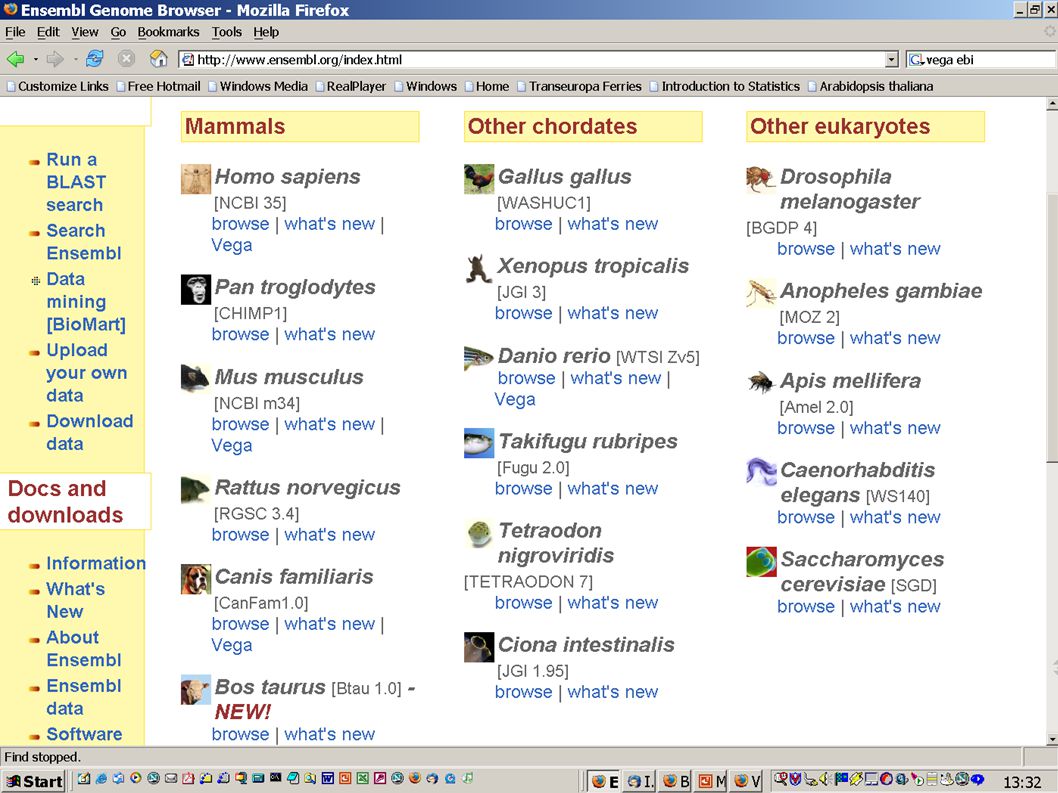
33. Ensembl martview

35. VEGA The Vertebrate Genome Annotation (VEGA) database is a central repository for high quality, frequently updated, manual annotation of vertebrate finished genome sequence. Current release: Human Mouse Zebrafish Dog http://vega.sanger.ac.uk

36. WormBase WormBase is the repository of mapping, sequencing and phenotypic information for C. elegans (and some other nematodes). http://www.wormbase.org

37. WormMart

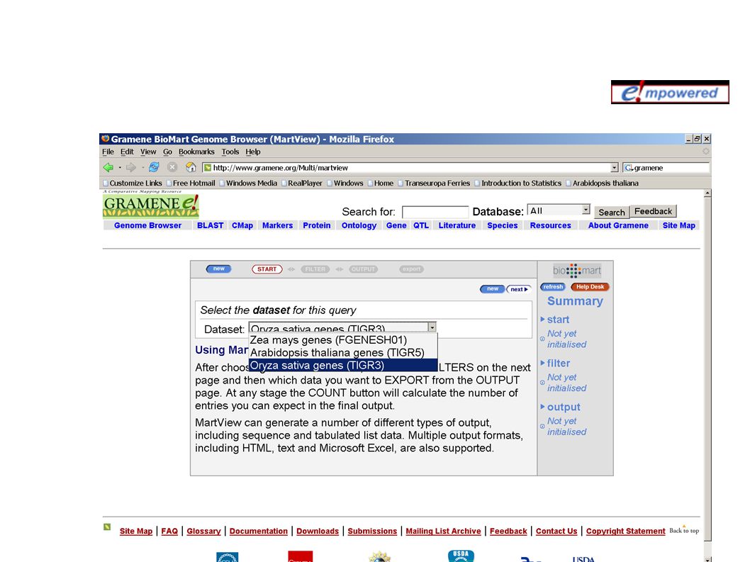
38. GrameneMart Gramene is a curated, open-source, Web-accessible data resource for comparative genome analysis in the grasses. http://www.gramene.org Gramene: A Comparative Mapping Resource for Grains

40. Other databases with BioMart interfaces dbSNP (via Ensembl)‏ HapMap Sequence Mart: Ensembl genome sequences

41. BioMart user interfaces

42. MartShell MartShell is a command line BioMart user interface based on a structured query language: Mart Query Language (MQL)‏

43. BioMart user interfaces Martview Web based user interface for BioMart, provides functionality for remote users to query all databases hosted by the EBI's public BioMart server. MartExplorer Perl and Java libraries biomaRt interface to R/Bioconductor

44. The biomaRt package Developed by Steffen Durinck (started Feb 2005) Two main sets of functions: 1. Tailored towards Ensembl, shortcuts for FAQs (frequently asked queries): getGene, getGO, getOMIM... 2. Generic queries, modeled after MQL (Mart query language), can be used with any BioMart dataset Two communication protocols 1. Direct MySQL queries to BioMart database servers 2. HTTP queries to BioMart webservices more stable (across database releases); self-reflective; less firewall problems

45. Getting started > library(biomaRt)‏ > listMarts()‏ $biomart [1] "dicty" "ensembl" "snp" "vega" "uniprot" "msd" "wormbase" $version [1] "DICTYBASE (NORTHWESTERN)" "ENSEMBL 38 (SANGER)" [3] "SNP 38 (SANGER)" "VEGA 38 (SANGER)" [5] "UNIPROT 4-5 (EBI)" "MSD 4 (EBI)" [7] "WORMBASE CURRENT (CSHL)" $host [1] "www.dictybase.org" "www.biomart.org" "www.biomart.org" [4] "www.biomart.org" "www.biomart.org" "www.biomart.org" [7] "www.biomart.org" $path [1] "" "/biomart/martservice" "/biomart/martservice" [4] "/biomart/martservice" "/biomart/martservice" "/biomart/martservice" [7] "/biomart/martservice"

46. Gene annotation The function getGene allows you to get gene annotation for many types of identifiers Supported identifiers are:  Affymetrix Genechip Probeset ID  RefSeq  Entrez-Gene  EMBL  HUGO  Ensembl  soon Agilent identifiers will also be available

47. getGene > mart <- useMart("ensembl", dataset = "hsapiens_gene_ensembl")‏ > myProbes <- c("210708_x_at", "202763_at", "211464_x_at")‏ > z <- getGene(id = myProbes, array = "affy_hg_u133_plus_2", mart = mart)‏ ID symbol 1 202763_at CASP3 2 210708_x_at CASP10 7 211464_x_at CASP6 description 1 Caspase-3 precursor (EC 3.4.22.-) (CASP-3) (Apopain)... 2 Caspase-10 precursor (EC 3.4.22.-) (CASP-10) (ICE-like apoptotic pro.. 7 Caspase-6 precursor (EC 3.4.22.-) (CASP-6) (Apoptotic protease Mch-2)... chromosome band strand chromosome_start chromosome_end ensembl_gene_id 1 4 q35.1 -1 185785845 185807623 ENSG00000164305 2 2 q33.1 1 201756100 201802372 ENSG00000003400 7 4 q25 -1 110829234 110844078 ENSG00000138794 ensembl_transcript_id 1 ENST00000308394 2 ENST00000272879 7 ENST00000265164

48. Gene annotation Note: Ensembl does an independent mapping of affy probe sequences to genomes. If there is no clear match then that probe is not assigned to a gene.

49. Gene annotation getGene returns a dataframe  Gene symbol  Description  Chromosome name  Band  Start position  End position  BioMartID

50. getGene > getGene(id = 100, type = "entrezgene", mart = mart)‏ ID symbol 1 100 ADA description 1 Adenosine deaminase (EC 3.5.4.4) (Adenosine aminohydrolase). [Source:Uniprot/SWISSPROT;Acc:P00813] chromosome band strand chromosome_start chromosome_end ensembl_gene_id 1 20 q13.12 -1 42681577 42713797 ENSG00000196839 ensembl_transcript_id 1 ENST00000372874

51. Other functions getGO: GO id, GO term, evidence code getOMIM (Online Mendelian Inheritance in Man, a catalogue of human genes and genetic disorders): OMIM id, Disease, BioMart id getINTERPRO (an integrated resource of protein families, domains and functional sites): Interpro id, description getSequence getSNP getHomolog

52. getSequence > seq <- getSequence(species="hsapiens", chromosome = 19, start = 18357968, end = 18360987, mart = mart) chromosome [1] "19" start [1] 18357968 end [1] 18360987 sequence "AGTCCCAGCTCAGAGCCGCAACCTGCACAGCCATGCCCGGGCAAGAACTCAGGACGGTGAATGGCTCTCAG ATGCTCCTGGTGTTGCTGGTGCTCTCGTGGCTGCCGCATGGGGGCGCCCTGTCTCTGGCCGAGGCGAGCCGC GCAAGTTTCCCGGGACCCTCAGAGTTGCACTCCGAAGACTCCAGATTCCGAGAGTTGCGGAAACGCTACGAG GACCTGCTAACCAGGCTGCGGGCCAACCAGAGCTGGGAAGATTCGAACACCGACCTCGTCCCGGCCCCTGCA GTCCGGATACTCACGCCAGAAGGTAAGTGAAATCTTAGAGATCCCCTCCCACCCCCCAAGCAGCCCCCATAT CTAATCAGGGATTCCTCATCTTGAAAAGCCCAGACCTACCTGCGTATCTCTCGGGCCGCCCTTCCCGAGGGG CTCCCCGAGGCCTCCCGCCTTCACCGGGCTCTGTTCCGGCTGTCCCCGACGGCGTCAAGGTCGTGGGACGTG ACACGACCGCTGCGGCGTCAGCTCAGCCTTGCAAGACCCCAGGCGCCCGCGCTGCACCTGCGACTGTCGCCG CCGCCGTCGCAGTCGGACCAACTGCTGGCAGAATCTTCGTCCGCACGGCCCCAGCTGGAGTTGCACTTGCGG CCGCAAGCCGCCAGGGGGCGCCGCAGAGCGCGTGCGCGCAACGGGGACCACTGTCCGCTCGGGCCCGGGCGT TGCTGCCGTCTGCACACGGTCCGCGCGTCGCTGGAAGACCTGGGCTGGGCCGATTGGGTGCTGTCGCCACGG GAGGTGCAAGTGACCATGTGCATCGGCGCGTGCCCGAGCCAGTTCCGGGCGGCAAACATG....

53. SNP Single Nucleotide Polymorphisms (SNPs) are common DNA sequence variations among individuals. e.g. AAGGCTAA and ATGGCTAA biomaRt uses the SNP mart of Ensembl which is obtained from dbSNP

54. getSNP > getSNP(chromosome = 8, start = 148350, end = 148612, mart = mart)‏ tsc refsnp_id allele chrom_start chrom_strand 1 TSC1723456 rs3969741 C/A 148394 1 2 TSC1421398 rs4046274 C/A 148394 1 3 TSC1421399 rs4046275 A/G 148411 1 4 rs13291 C/T 148462 1 5 TSC1421400 rs4046276 C/T 148462 1 6 rs4483971 C/T 148462 1 7 rs17355217 C/T 148462 1 8 rs12019378 T/G 148471 1 9 TSC1421401 rs4046277 G/A 148499 1 10 rs11136408 G/A 148525 1 11 TSC1421402 rs4046278 G/A 148533 1 12 rs17419210 C/T 148533 -1 13 rs28735600 G/A 148533 1 14 TSC1737607 rs3965587 C/T 148535 1 15 rs4378731 G/A 148601 1

55. Homology mapping The getHomolog function enables mapping of many types of identifiers from one species to the same or another type of identifier in another species.

56. getHomolog > from.mart = useMart("ensembl", dataset = "hsapiens_gene_ensembl")‏ > to.mart = useMart("ensembl", dataset = "mmusculus_gene_ensembl")‏ > getHomolog(id = 2, from.type = "entrezgene", to.type = "refseq", + from.mart = from.mart, to.mart = to.mart)‏ V1 V2 V3 1 ENSMUSG00000030111 ENSMUST00000032203 NM_175628 2 ENSMUSG00000059908 ENSMUST00000032228 NM_008645 3 ENSMUSG00000030131 ENSMUST00000081777 NM_008646 4 ENSMUSG00000071204 ENSMUST00000078431 NM_001013775 5 ENSMUSG00000030113 ENSMUST00000032206 6 ENSMUSG00000030359 ENSMUST00000032510 NM_007376

57. Find (microarray) probes of interest getFeature function Filter on: gene location symbol OMIM GO

58. getFeature > getFeature(symbol = "BRCA2", array = "affy_hg_u133_plus_2", mart = mart)‏ hgnc_symbol affy_hg_u133_plus_2 1 BRCA2 208368_s_at > getFeature(chromosome = 1, start = 2800000, end = 3200000, type = "entrezgene", + mart = mart)‏ ensembl_transcript_id chromosome_name start_position end_position entrezgene 1 ENST00000378404 1 2927907 2929327 140625 2 ENST00000304706 1 2927907 2929327 140625 3 ENST00000321336 1 2970496 2974193 440556 4 ENST00000378398 1 2975621 3345045 63976 5 ENST00000378398 1 2975621 3345045 647868 6 ENST00000270722 1 2975621 3345045 63976 7 ENST00000270722 1 2975621 3345045 647868 8 ENST00000378391 1 2975621 3345045 63976 9 ENST00000378391 1 2975621 3345045 647868 10 ENST00000378389 1 2975621 3345045 NA 11 ENST00000378388 1 2975621 3345045 NA

59. getFeature Select all RefSeq id’s involved in diabetes mellitus: >getFeature(OMIM="diabetes mellitus", type="refseq", species="hsapiens", mart=mart) ‏

60. Ensembl Cross-references Powerful function to map between all possible cross-references in Ensembl Can for example be used to map between different Affymetrix arrays

61. Ensembl Cross-references getPossibleXrefs  Retrieves all possible cross-references > xref <- getPossibleXrefs(mart = mart)‏ > xref[1:10, ] species xref [1,] "agambiae" "embl" [2,] "agambiae" "pdb" [3,] "agambiae" "prediction_sptrembl" [4,] "agambiae" "protein_id" [5,] "agambiae" "uniprot_accession" [6,] "agambiae" "uniprot_id"

62. Ensembl Cross-references >xref = getXref(id="1939_at", from.species="hsapiens", to.species = "mmusculus", from.xref = "affy_hg_u95av2", to.xref = "affy_mouse430_2", mart=mart)‏

63. The generic interface: the getBM function

64. useDataset > library(biomaRt)‏ > mart <- useMart("ensembl")‏ > listDatasets(mart)‏ dataset version 1 rnorvegicus_gene_ensembl RGSC3.4 2 scerevisiae_gene_ensembl SGD1 3 celegans_gene_ensembl CEL150 4 cintestinalis_gene_ensembl JGI2 5 ptroglodytes_gene_ensembl CHIMP1A 6 frubripes_gene_ensembl FUGU4 7 agambiae_gene_ensembl AgamP3 8 hsapiens_gene_ensembl NCBI36 9 ggallus_gene_ensembl WASHUC1 10 xtropicalis_gene_ensembl JGI4.1 11 drerio_gene_ensembl ZFISH5....(more)... > mart <- useDataset(dataset = "hsapiens_gene_ensembl", mart = mart)‏

65. getBM > getBM(attributes = c("affy_hg_u95av2", "hgnc_symbol"), filter = "affy_hg_u95av2", values = c("1939_at", "1000_at"), mart = mart)‏ affy_hg_u95av2 hgnc_symbol 1 1000_at MAPK3 3 1939_at TP53 mart – an object describing the database connection and the dataset attributes – the name of the data you want to obtain filter – the name of the data by which you want to filter from the dataset values – values to filter on

66. Locally installed BioMarts Main use case currently is to use biomaRt to query public BioMart servers over the internet But you can also install BioMart server locally, populated with a copy of a public dataset (particular version), or populated with your own data Versioning is supported by naming convention

67. Installation bioMart depends on R packages Rcurl, XML, which require additional system libraries (libcurl, libxml2)‏ RMySQL package is optional Platforms on which biomaRt has been installed: Linux Mac OS X Windows

68. Discussion Using biomaRt to query public webservices gets you started quickly, is easy and gives you access to a large body of metadata in a uniform way Need to be online Online metadata can change behind your back; although there is possibility of connecting to a particular, immutable version of a dataset Watch this space – implementation of Bioconductor metadata packages is changing and improving! using the familiar packaging and versioning system