Download presentation
Presentation is loading. Please wait.

1
Tracers in Ocean and Climate Models* Matthew England CEMAP, School of Mathematics The University of New South Wales * See also www.maths.unsw.edu.au/~matthew/publications.html#MR98

3
Possible due to: GEOSECS, TTO, SAVE, WOCE, …..

5
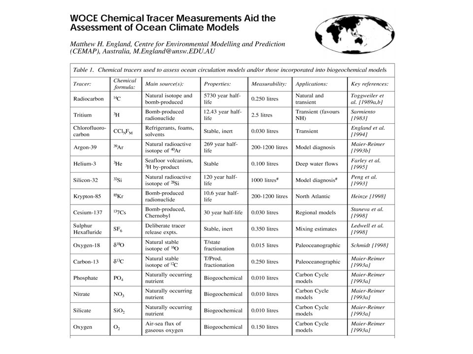
Why bother with tracers in models? Ocean model “validation” Diagnosis of model circulation mechanisms Studies of the ocean carbon cycle Data assimilation studies Paleoceanographic considerations

6
Ocean model “validation” (e.g. CFCs, 14 C) Diagnosis of model circulation mechanisms (e.g. dye/age tracers, 39 Ar) Studies of the ocean carbon cycle (carbon compounds, oxygen, phosphate, nitrate,…) Data assimilation studies (e.g. CFCs, tritium) Paleoceanographic considerations (e.g. carbon-13, oxygen-18) Why bother with tracers in models?
 Studies of the ocean carbon cycle (carbon compounds, oxygen, phosphate, nitrate,…) Data assimilation studies (e.g. CFCs, tritium) Paleoceanographic considerations (e.g. carbon-13, oxygen-18) Why bother with tracers in models .")
7
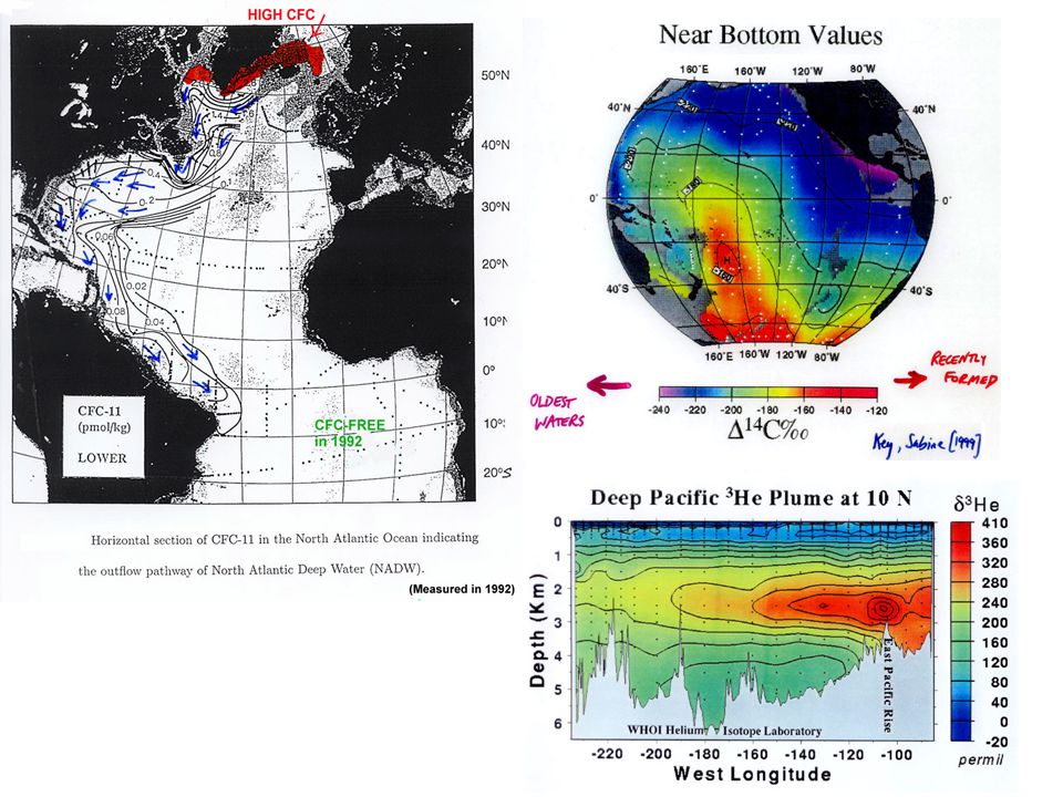
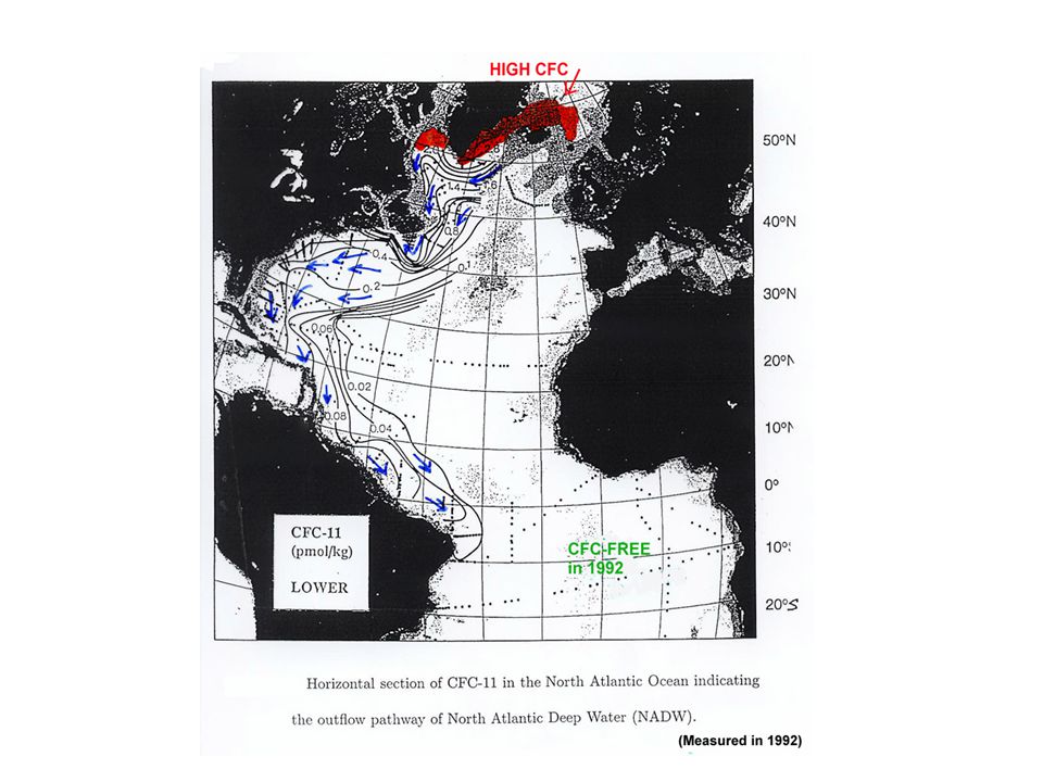
100-1000 year ventilation 10-100 year ventilation

8
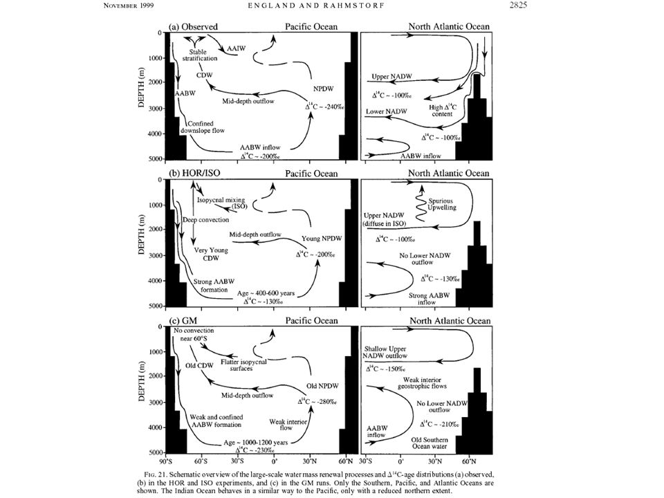
Robust diagnostic: T-S restored to observed in the interior Robust diagnosticObserved 14C Prognostic Supressed convection and vertical motion Prognostic experiment: Interior T-S free to evolve Toggweiler et al. [1989]

10
Chlorofluorocarbons

12
Plate 2. Distribution of CFC-12 on isopycnal surfaces corresponding to maximum NADW outflow in 1988 in the Redler and Dengg [1999] simulations. (a) In the 4/3° model, and (b) in the 1/3° model. The color bar indicates CFC concentrations in pmol/kg, with isopycnal layer depths contoured (meters).
 In the 4/3° model, and (b) in the 1/3° model. The color bar indicates CFC concentrations in pmol/kg, with isopycnal layer depths contoured (meters)..")
13
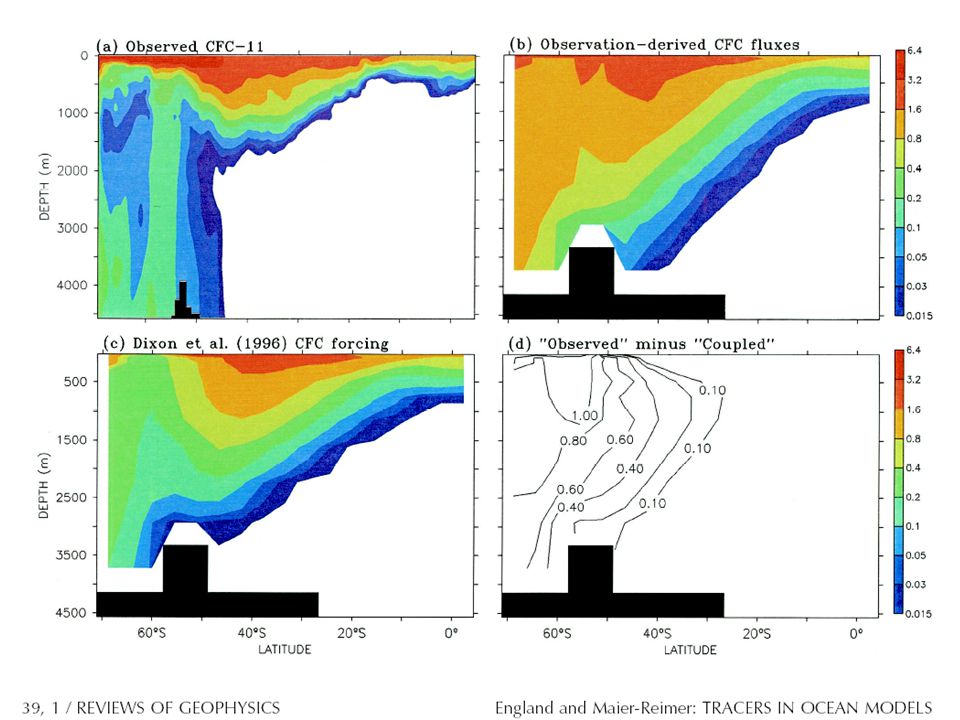
Ajax section in the South Atlantic CDW AAIW AABW

14
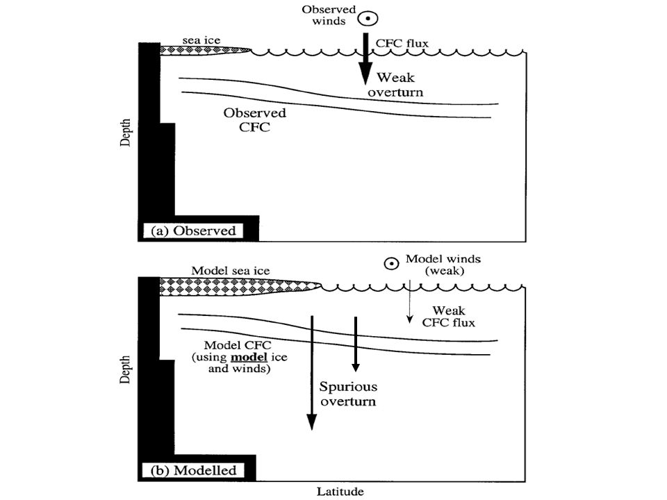
Forcing functions for tracers ? sea-ice CFC 14 C 3 He CFC 14 C 3 He CFC 14 C CFC 14 C CFC 14 C CFC Air-sea gas flux = f (k, ice, ) k = piston velocity ~ wind speed, U 2 or U 3 = solubility ~ SST, (SSS)
 k = piston velocity ~ wind speed, U 2 or U 3 = solubility ~ SST, (SSS).")
15
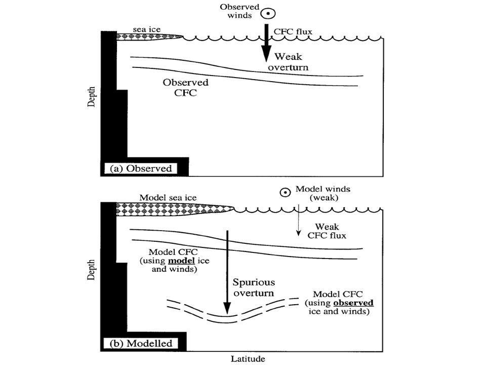
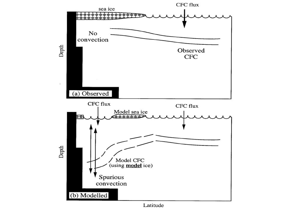
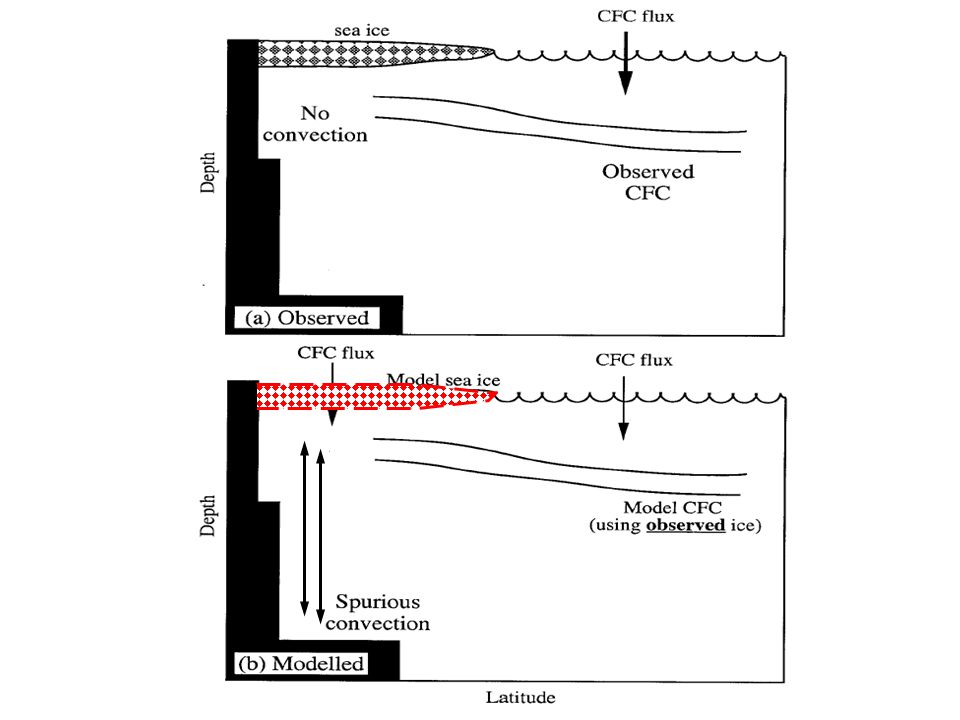
How to compute gas uptake: Use model-generated ice, winds, T-S? Use observed ice, winds, T-S? Tracers in coupled climate models: Both approaches can give an apparently good tracer simulation but for the wrong reason (see England and Maier-Reimer 2001 for details)
.")
16
Case 1:

20
Spurious convection Case 2:

23
Other tracer techniques: Age/Dye tracers Tracer data assimilation Off-line tracer models (Cox, 1989, England 1995, O’Farrell 2000….) (Haine 1999, Schlitzer 1996, …) (Aumont 1998, Sen Gupta & England 2003)
 (Haine 1999, Schlitzer 1996, …) (Aumont 1998, Sen Gupta & England 2003)")
24
Off-Line Tracer Model Tracer Conservation Equation OGCM Horizontal Velocity Fields Source Terms Mixing Terms Tracer Concentration T (x, y, z, t) Continuity Equation u, vw Interannual Seasonal Intraseasonal Water-mass source regions CFCs, 14 C, 3 He Radioactive waste T, S Pollution, etc…. Eddy statistics Isopycnal mixing GM (1990) Convective ML Wind Driven ML T, S, CFCs, 14 C,….
 Convective ML Wind Driven ML T, S, CFCs, 14 C,…..")
25
PhD project: Alex Sen Gupta Example: CFC simulations in a ¼ degree model Integrated CFC content below 2000m Year = 1980

26
PhD project: Alex Sen Gupta Integrated CFC content below 2000m Year = 2000

27
PhD project: Alex Sen Gupta Integrated CFC content below 2000m Year = 2020

28
PhD project: Alex Sen Gupta Integrated CFC content below 2000m Year = 2040

29
Advantages: Independent assessment of model (complements T-S) Can validate within ocean-only component Complements GBC and carbon cycle modelling Drawbacks: Extra CPU (especially 14 C) Can manipulate outcome to some extent Uncertainties: Tracer source functions Sparse data How to formalise assessment? Summary – Tracers in climate models

Similar presentations
>")


 Water mass analysis.>")

 basin.>")


 Fall 2014>")
 –basin.>")

 at NCEP>")
