2. Pro Forma Analysis Agribusiness Finance LESE 306 Fall 2009

3. PASTFUTURE PRESENT  Historical analysis  Comparative analysis  Historical price and yield trends  Pro forma analysis  Forming expectations about future prices, costs and productivity  Ad hoc extrapolations  Projections based upon available outlook data  Projections based upon econometric analysis

4. 2009 2010 2011 2012 2013 2014 2015 Timeline Required for Capital Budgeting… Assume it is the year 2009 and John Deere wants to project farm machinery and equipment sales over the next six years to determine if plant expansion is necessary.

5. 2009 2010 2011 2012 2013 2014 2015 Timeline Required for Capital Budgeting… Assume it is the year 2009 and John Deere wants to project farm machinery and equipment sales over the next six years to determine if plant expansion is necessary. Capital budgeting models of investment decisions require projections of the annual revenue and cost values over the entire 2010 to 2015 time period. Page 89 in booklet

6. Page 74 in booklet Remember the definition of annual net cash flows

7. Page 85 in booklet Must project Annual price Must project Annual price Must project Annual yield Must project Annual yield

8. Alternative Forecasting Approaches

9. Ad Hoc Modeling Approaches Naïve model – using last year’s prices, costs and yields Simple linear trend extrapolation of historical prices, costs and yields Moving Olympic average Using assumptions made by others

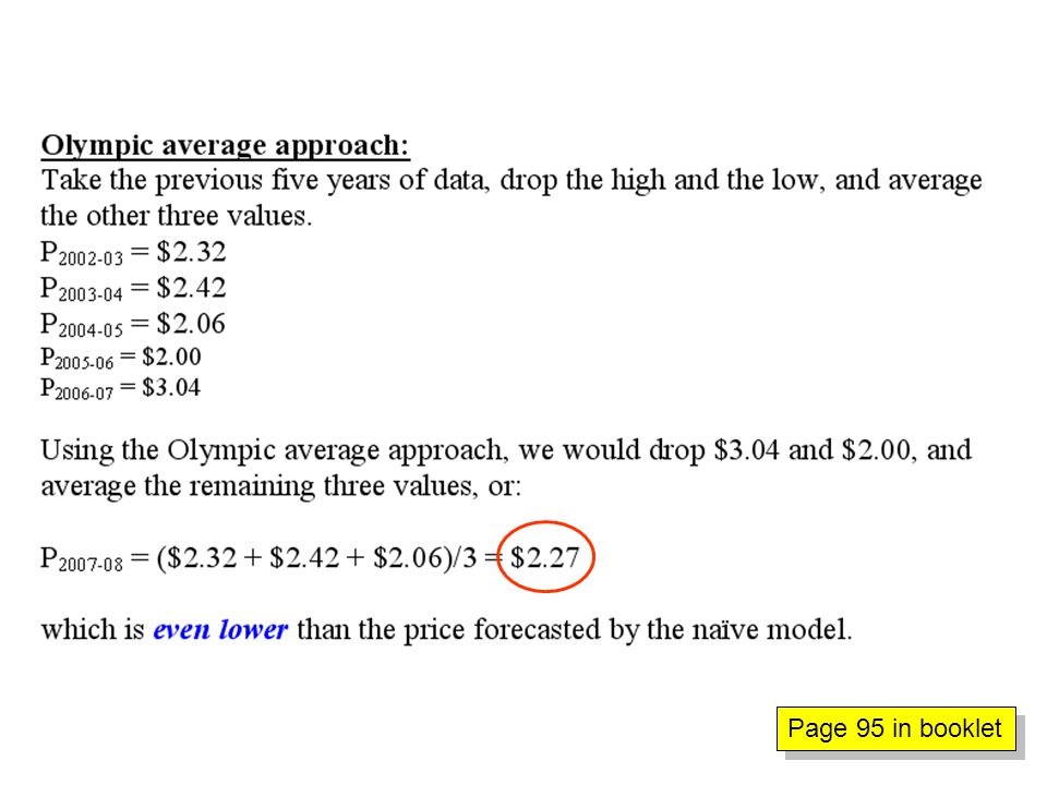
10. Naïve model: P t = P t-1 Linear trend: P t = a 0 + a 1 (Year) Olympic average: P t = Last 5 year annual price, dropping high and low and calculate the average of the remaining three year’s price. Ad Hoc Modeling Approaches

11. Page 94 in booklet

13. Page 95 in booklet

14. Econometric Model Approach Capturing future supply/demand impacts on prices and unit costs Linkages to commodity policy Linkages to domestic economy Linkages to the global economy

15. Concept of Derived Demand for Farm Machinery The demand for farm machinery is driven by the expected net economic benefit from use of the machine….

16. Crop Market Equilibrium D S D S Quantity Price PePe QeQe D S Demand consists of: -Industrial use -Feed use -Exports -Ending stocks Demand consists of: -Industrial use -Feed use -Exports -Ending stocks Supply consists of: -Beginning stocks -Production -Imports Supply consists of: -Beginning stocks -Production -Imports Page 45 in booklet

17. Forecasting Future Commodity Price Trends D S $4 10 $1 $7 D = a – bP + cYD + eX Own price Own price Disposable income Disposable income Other factors Other factors Page 45 in booklet

18. D S $4 10 $1 $7 S = n + mP – rC + sZ Own price Own price Input costs Input costs Forecasting Future Commodity Price Trends Other factors Other factors Page 46 in booklet

19. Projecting Commodity Price D = S D S $4 10 $1 $7 D = 10 – 6P +.3YD + 1.2X S = 2 + 4P –.2C + 1.02Z Substitute the demand and supply equations into the the equilibrium condition and solve for price Substitute the demand and supply equations into the the equilibrium condition and solve for price Page 46 in booklet

20. The Market Model Demand equations: Q d,i = a 0 - a 1 (Price) +  a i (demand shifters) Supply equation: Q s,i = b 0 +b 1 (price) +  b i (supply shifters) Market equilibrium: ΣQ d,i = ΣQ s,i

21. An Example

22. Historical Data on Fixed Input Sales to Farmers

23. Econometric Analysis Based on Time Trend Extrapolation I t = f(Year t )

24. poor job A linear time trend projection of future farm machinery and equipment sales therefore does a poor job of predicting future sales activity.

25. Econometric Analysis Based on Investment Theory Econometric Analysis Based on Investment Theory I t = f{[E(P t )×E(Q t )]/E(c t )} Incorporates the economic concepts of MVP and MIC

26. muchbetter job An econometric model based on investment theory does a much better job of predicting future sales activity.

27. Another Example

28. Estimating the Annual Supply and Use of Wheat

29. Income elasticity Cross price elasticity Econometric Analysis – Food Use Own price elasticity

30. Observed and Predicted Values For Wheat Food Use

31. Remaining Steps to Forecasting the Price of Commodity Develop similar econometric equations for the other uses of wheat (feed use, exports and ending stock). Develop econometric equations for production and import supply. (Q D =Q S ) solve for the price whereexcess demand equals zero Substitute the estimated equations into the market equilibrium definition (Q D =Q S ) and solve for the price where excess demand equals zero.

32. Stress Testing Your Forecast

33. PEPE QEQE Assumes perfect knowledge of outcomes in all 5 areas!!!! Point Forecast Assumptions Page 47 in booklet

34. Supply-side risk for a given price… QLQEQHQLQEQH PEPE Structural Pro Forma Analysis Page 47 in booklet

35. Demand and supply- side risk and potential price variability… QLQEQHQLQEQH PHPEPLPHPEPL Structural Pro Forma Analysis Page 47 in booklet

36. Page 85 in booklet A 48 percent chance that the price of wheat will be less than $4.16

37. Page 96 in booklet Potential Variability in Wheat Price 2008/09 MY Given Historical Variability in Growing Conditions Ratings

38. Page 93 in booklet

39. Triangular Probability Distribution $2.50 $3.00 $3.50 Page 131 in booklet

40. Conclusions Econometric models preferred over naïve models and linear time trend models. Much more accurate. elasticities Provide much more information (e.g., elasticities). sensitivity analysis potential variability Allow for sensitivity analysis with independent (exogenous) variables when evaluating potential variability about expected trends.

41. NCF Summary

42. Page 74 in booklet

43. Page 82 in booklet

44. G is the expected rate of appreciation

45. Page 79 in booklet Allowing for unequal annual net cash flows….

46. Page 63 in booklet Allowing for unequal discount rates…

47. Concept of Required Rate of Return

48. Adjusting Discount Rate We said to date that the discount rate is the firm’s opportunity rate of return. Realistically we must allow for business risk by including a risk premium. Realistically we must also allow for financial risk by adding an additional risk premium.

49. Business Risk price Risk associated with price of the product or products you are producing. unit costs Risk associated with the unit costs for the inputs used in producing the product(s). yields Risk associated with yields (productivity) in production. NCF i =P i  yields i  unit sales – C i  unit inputs

50. Accounting for Business Risk R FREE,i = risk free rate of return (i.e., govt. bond rate) RRR L,i = required rate of return for lowly risk averse RRR H,i = required rate of return for highly risk averse R FREE,i RRR L,i RRR H,i.05 Page 132 in booklet

51. Increasing Risk Over Time Expected price Expected price E(P) Year 1 Year 10 Pessimistic price Pessimistic price Optimistic price Optimistic price Product price distribution Product price distribution $2.95 $3.05 $3.15 Probability

52. Increasing Risk Over Time Expected price Expected price E(P) Year 1 Year 10 Pessimistic price Pessimistic price Optimistic price Optimistic price Product price distribution Product price distribution $2.05 $2.95 $3.05 $3.15 $4.05 Probability

53. Financial Risk Risk associated with low used borrowing capacity (remember we captures this in the implicit cost of capital). Risk associated with increasing explicit cost of debt capital relative to ROA. We discussed this when analyzing the economic growth model: ROE = [(r – i)L + r](1 – tx)(1 – w)

54. Accounting for Financial Risk R FREE,i RRR i.05 Page 138 in booklet

55. Required Rate of Return For the purposes of this course, we will measure the annual required rates of return based upon a subjective methods. Ask yourself what additional return you require above a risk-free rate given your perceived annual business risk. Ask yourself what additional return you require given existing leverage position. RRR i = R free,i + R business,i + R financial,i

56. One Strategy to Minimizing Risk Exposure Page 140 in booklet

57. Forecast horizon NCF i NCF with existing assets NCF with new assets The Portfolio Effect

58. Forecast horizon NCF i Average annual NCF after making new investment. The Portfolio Effect This allows use to lower the business risk premium associated with the calculated the NPV for the new investment project. Exchanging stable profits for lowering exposure to risk.

59. Our Final NPV Model

60. Page 63 in booklet Allowing for unequal annual net cash flows and required rates of return….

61. NPV = NCF 1 [1/(1+R 1 )] + NCF 2 [1/(1+R 1 )(1+R 2 )] + … + NCF n [1/(1+R 1 )(1+R 2 )…(1+R n )] + T[1/(1+R 1 )(1+R 2 )…(1+R n )] – tx(T – C)[1/(1+R 1 )(1+R 2 )…(1+R n )] Our Complete NPV Capital Budgeting Model Discounted NCF in year 1 Discounted NCF in year 2 Discounted NCF in year n Discounted terminal value Discounted capital gains tax NPV > 0 suggests project is economically feasible NPV = 0 suggests indifference NPV < 0 suggests project is economically infeasible Decision rule:

62. Ranking Investment Opportunities

63. Page 106 in booklet

64. * *

65. Page 107 in booklet * *

67. Page 108 in booklet

68. Borrowing Preparation 1.Up to date financial statements. 2.Demonstrate trends in key financial ratios including debt repayment coverage. 3.Pro forma master budget before and after proposed investment, including the line of credit or LOC. 4.Do sensitivity analysis. 5.Demonstrate feasibility of investment plans by using NPV capital budgeting using stress testing and incorporation of risk.

69. Both Sides of the Desk The borrower: Enterprise analysis Cash management Line of credit needs Operating loan application Investment planning Term loan application Planning for long run Coverage thus far this semester

70. Both Sides of the Desk The borrower: Enterprise analysis Cash management Line of credit needs Operating loan application Investment planning Term loan application Planning for long run The lender: Loan application analysis Credit scoring Loan pricing for risk Loan approval process Loan portfolio analysis Loan loss reserves Regulatory oversight Lending institutions serving commercial agriculture and rural businesses. After mid-term exam