1. Multiple Investment Alternatives Sensitivity Analysis

2. Given two or more investment alternatives, be able to identify the mutually exclusive alternatives. Given two or more mutually exclusive investment alternatives, be able to determine the best alternative by the present worth method the annual worth method the incremental rate-of-return Given a problem description, be able the breakeven point between two or more investment alternatives. Given a cash flow, be able to perform a sensitivity analysis on one or two parameters of the cash flow.

3. NPW > 0 Good Investment EUAW > 0 Good Investment IRR > MARR Good Investment Note: If NPW > 0 EUAW > 0 IRR > MARR

4. NPW A > NPW B Choose A Must use same planning horizon EUAW A > EUAW B Choose A Same Planning Horizon implicit in computation IRR A > IRR B Choose A Must use Incremental Rate-of-Return IRR B-A < MARRChoose A

5. Suppose we have two projects, A & B A B Initial cost$50,000$80,000 Annual maintenance 1,000 3,000 Increased productivity 10,000 15,000 Life 10 10 Salvage 10,000 20,000

6. A NPW(10) = -50 + 9(P/A,10,10) + 10(P/F,10,10) 50 9 9 10 0 123...

7. A NPW(10) = -50 + 9(P/A,10,10) + 10(P/F,10,10) = -50 + 9(6.1446) + 10(.3855) 50 9 9 10 0 123...

8. A NPW(10) = -50 + 9(P/A,10,10) + 10(P/F,10,10) = -50 + 9(6.1446) + 10(.3855) = $9,156 50 9 9 10 0 123...

9. B 80 12 20 0 12310... NPW(10) = -80 + 12(P/A,10,10) + 20(P/F,10,10)

10. B 80 12 20 0 12310... NPW(10) = -80 + 12(P/A,10,10) + 20(P/F,10,10) = -80 + 12(6.1446) + 20(.3855)

11. B 80 12 20 0 12310... NPW(10) = -80 + 12(P/A,10,10) + 20(P/F,10,10) = -80 + 12(6.1446) + 20(.3855) = $1,445

12. NPW A > NPW B Choose A

13. 50 9 9 10 0 123... A EUAW(10) = -50(A/P,10,10) + 9 + 10(A/F,10,10)

14. 50 9 9 10 0 123... A EUAW(10) = -50(A/P,10,10) + 9 + 10(A/F,10,10) = -50 (.1627) + 9 + 10(.0627)

15. 50 9 9 10 0 123... A EUAW(10) = -50(A/P,10,10) + 9 + 10(A/F,10,10) = -50 (.1627) + 9 + 10(.0627) = $1,492

16. 12 20 0 12310... B EUAW(10) = -80(A/P,10,10) + 12 + 20(A/F,10,10)

17. 12 20 0 12310... B EUAW(10) = -80(A/P,10,10) + 12 + 20(A/F,10,10) = -80(.1627) + 12 + 20(.0627)

18. 12 20 0 12310... B EUAW(10) = -80(A/P,10,10) + 12 + 20(A/F,10,10) = -80(.1627) + 12 + 20(.0627) = $238

19. EUAW A > EUAW B Choose A

20. Example: Suppose MARR is 10%. Suppose also that we can invest in T-bill @15% or we can invest in a 5 year automation plan. 100 115 NPW = 115(1.1) -1 - 100 = $4,545 100 30 51234 NPW = 30(P/A,10,5) - 100 = $13,724 AB B

21. But this ignores reinvestment of T-bills for full 5-year period. 0 5 100 201,135 NPW = 201.135(P/F,10,5) - 100 = $24,889 A

22. Projects must be compared using same Planning Horizon

23. 4,000 3 3,500 4,500 A NPW = -4 + 3.5(P/A, 10,3) + 4.5(P/F,10,3)

24. 4,000 3 3,500 4,500 A NPW = -4 + 3.5(P/A, 10,3) + 4.5(P/F,10,3) = -4 + 3.5(2.4869) + 4.5(.7513)

25. 4,000 3 3,500 4,500 A NPW = -4 + 3.5(P/A, 10,3) + 4.5(P/F,10,3) = -4 + 3.5(2.4869) + 4.5(.7513) = 8.085 = $8,085

26. 5,000 3 3,000 5,000 6 B NPW= -5 + 3(P/A,10,6) + 5(P/F,10,6)

27. 5,000 3 3,000 5,000 6 B NPW= -5 + 3(P/A,10,6) + 5(P/F,10,6) = -5 + 3(4.3553) + 5(.5645)

28. 5,000 3 3,000 5,000 6 B NPW= -5 + 3(P/A,10,6) + 5(P/F,10,6) = -5 + 3(4.3553) + 5(.5645) = 10.888 = $10,888

29. Least Common Multiple Shortest Life Longest Life Standard Planning Horizon

30. A 4,000 3 3,500 4,500 4,000 6 4,500 NPW= -4 -4(P/F,10,3) + 3.5(P/A,10,6) + 4.5(P/F,10,3) + 4.5(P/F,10,6)

31. A 4,000 3 3,500 4,500 4,000 6 4,500 NPW= -4 -4(P/F,10,3) + 3.5(P/A,10,6) + 4.5(P/F,10,3) + 4.5(P/F,10,6) = -4 +.5(P/F,10,3) + 3.5(P/A,10,6) + 4.5(P/F,10,6)

32. A 4,000 3 3,500 4,500 4,000 6 4,500 NPW= -4 -4(P/F,10,3) + 3.5(P/A,10,6) + 4.5(P/F,10,3) + 4.5(P/F,10,6) = -4 +.5(P/F,10,3) + 3.5(P/A,10,6) + 4.5(P/F,10,6) = -4 +.5(.7513) + 3.5(4.3553) + 4.5(.5645)

33. A 4,000 3 3,500 4,500 4,000 6 4,500 NPW= -4 -4(P/F,10,3) + 3.5(P/A,10,6) + 4.5(P/F,10,3) + 4.5(P/F,10,6) = -4 +.5(P/F,10,3) + 3.5(P/A,10,6) + 4.5(P/F,10,6) = -4 +.5(.7513) + 3.5(4.3553) + 4.5(.5645) = 14.159 = $14,159

34. 5,000 3 3,000 5,000 6 B NPW= -5 + 3(P/A,10,6) + 5(P/F,10,6)

35. 5,000 3 3,000 5,000 6 B NPW= -5 + 3(P/A,10,6) + 5(P/F,10,6) = -5 + 3(4.3553) + 5(.5645)

36. 5,000 3 3,000 5,000 6 B NPW= -5 + 3(P/A,10,6) + 5(P/F,10,6) = -5 + 3(4.3553) + 5(.5645) = 10.888 = $10,888

37. NPW A > NPW B Choose A

38. 4,000 3 3,500 4,500 A EUAW = -4(A/P,10,3) + 3.5 + 4.5(A/F,10,3) = -4(.4021) + 3.5 + 4.5(.3021) = 3.251 = $3,251 Note: NPW = 3,251(P/A,10,6) = 3,251(4.3553) = $14,159

39. 5,000 3 3,000 5,000 6 B EUAW = -5(A/P,10,6) + 3 + 5(A/F,10,6) = -5(.2296) + 3 + 5(.1296) = 2.500 = $2,500 Note: NPW = 2,500(P/A,10,6) = $10,888

40. Equivalent Uniform Annual Worth method implicitly assumes that you are comparing alternatives on a least common multiple planning horizon

41. Two alternatives for a recreational facility are being considered. Their cash flow profiles are as follows. Using a MARR of 10%, select the preferred alternative.

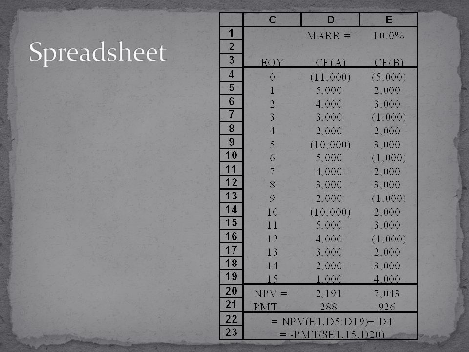
42. 1 2 3 4 5 11 5 4 3 2 1 EUAW A = -11(A/P,10,5) + 5 - 1(A/G,10,5) = -11(.2638) + 5 - 1(1.8101) =.2881 = $288

43. 1 2 3 5 4 3 2 EUAW B = -5(A/P,10,3) + 2 + 1(A/G,10,3) = -5(.4021) + 2 + 1(.9366) =.9261 = $926

44. EUAW B > EUAW A Choose B

45. 1 2 3 4 5 11 5 4 3 2 1 A B 1 2 3 5 4 3 2 Use Net Present Worth and least common multiple of lives to compare alternatives A & B.

46. 1 2 3 4 5 11 5 4 3 2 1 A B 1 2 3 5 4 3 2 Use Net Present Worth and least common multiple of lives to compare alternatives A & B. NPW A = 288(P/A,10,15) = 288(7.6061) = $2,191

47. 1 2 3 4 5 11 5 4 3 2 1 A B 1 2 3 5 4 3 2 Use Net Present Worth and least common multiple of lives to compare alternatives A & B. NPW A = 288(P/A,10,15) = 288(7.6061) = $2,191 NPW B = 926(P/A,10,15) = 926(7.6061) = $7,043

49. Suppose we have two investment alternatives A 100 110 1 IRR A = 10% B 200 226 1 IRR B = 13%

50. Suppose we have two investment alternatives AB 100 110 200 226 11 IRR A = 10%IRR B = 13% IRR B > IRR A Choose B

51. Suppose we have two investment alternatives AB 100 110 200 226 11 IRR A = 10%IRR B = 13% IRR B > IRR A Choose B

52. Investment alternative B costs $200. If we forego B for $100 invested in A, we have an extra $100 which can be invested at MARR. If MARR = 20%,

53. Investment alternative B costs $200. If we forego B for $100 invested in A, we have an extra $100 which can be invested at MARR. If MARR = 20%, A 100 110 1 IRR A = 15% + 100 120 1 = 200 230 1

54. B 200 226 1 IRR B = 13% IRR A > IRR B Choose A 200 230 1 A IRR A = 15%

55. Suppose we have $100,000 to spend and we have two mutually exclusive investment alternatives both of which yield returns greater than MARR = 15%. A 50,000 60,000 1 IRR A = 20% B 90,000 106,200 1 IRR B = 18%

56. A 50,000 60,000 1 IRR A = 20% B 90,000 106,200 1 IRR B = 18% IRR A > IRR B Choose A

57. A 50,000 60,000 1 IRR A = 20% B 90,000 106,200 1 IRR B = 18% IRR A > IRR B Choose A

58. A 50,000 60,000 1 NPW A = -50 + 60(1.15) -1 = $2,170 B 90,000 106,200 1 NPW B = -90 + 106.2(1.15) -1 = $2,350 NPW B > NPW A Choose B

59. Remember, we have $100,000 available in funds so we could spend an additional $50,000 above alternative A or an additional $10,000 above alternative B. If we assume we can make MARR or 15% return on our money, then

60. if we invest in A, we have an extra $50,000 which can be invested at MARR (15%). A 50,000 60,000 1 i = 20% 50,000 57,500 1 i = 15% += 100,000 117,500 1 i c = 17.5%

61. If we invest in B, we have an extra $10,000 which can be invested at MARR (15%). B 90,000 106,200 1 i = 18% 10,000 11,500 1 i = 15% += 100,000 117,700 1 i c = 17.7%

62. B 100,000 117,700 1 IRR B = 17.7% IRR cB > IRR cA Choose B 100,000 117,500 1 A IRR A = 17.5%

66. Break Even & Sensitivity

67. Suppose that by investing in a new information system, management believes they can reduce inventory costs. Your boss asks you to figure out if it should be done.

68. Suppose that by investing in a new information system, management believes they can reduce inventory costs. After talking with software vendors and company accountants you arrive at the following cash flow diagram. 1 2 3 4 5 100,000 25,000 i = 15%

69. Suppose that by investing in a new information system, management believes they can reduce inventory costs. After talking with software vendors and company accountants you arrive at the following cash flow diagram. 1 2 3 4 5 100,000 25,000 NPW = -100 + 25(P/A,15,5) = -16,196 i = 15%

70. Suppose that by investing in a new information system, management believes they can reduce inventory costs. After talking with software vendors and company accountants you arrive at the following cash flow diagram. 1 2 3 4 5 100,000 25,000 NPW = -100 + 25(P/A,15,5) = -16,196 i = 15%

71. Boss indicates $25,000 per year savings is too low & is based on current depressed market. Suggests that perhaps $40,000 is more appropriate based on a more aggressive market. 1 2 3 4 5 100,000 40,000

72. Boss indicates $25,000 per year savings is too low & is based on current depressed market. Suggests that perhaps $40,000 is more appropriate based on a more aggressive market. 1 2 3 4 5 100,000 40,000 NPW = -100 + 40(P/A,15,5) = 34,086

73. Boss indicates $25,000 per year savings is too low & is based on current depressed market. Suggests that perhaps $40,000 is more appropriate based on a more aggressive market. 1 2 3 4 5 100,000 40,000 NPW = -100 + 40(P/A,15,5) = 34,086

74. Tell your boss, new numbers indicate a go. Boss indicates that perhaps he was a bit hasty. Sales have fallen a bit below marketing forecast, perhaps a 32,000 savings would be more appropriate 1 2 3 4 5 100,000 32,000

75. Tell your boss, new numbers indicate a go. Boss indicates that perhaps he was a bit hasty. Sales have fallen a bit below marketing forecast, perhaps a 32,000 savings would be more appropriate 1 2 3 4 5 100,000 32,000 NPW = -100 + 32(P/A,15,5) = 7,269

76. Tell your boss, new numbers indicate a go. Boss indicates that perhaps he was a bit hasty. Sales have fallen a bit below marketing forecast, perhaps a 32,000 savings would be more appropriate 1 2 3 4 5 100,000 32,000 NPW = -100 + 32(P/A,15,5) = 7,269

77. Tell your boss, new numbers indicate a go. Boss leans back in his chair and says, you know....

78. I’ll do anything, just tell me what numbers you want to use!

79. 1 2 3 4 5 100,000 A NPW = -100 + A(P/A,15,5) > 0

80. 1 2 3 4 5 100,000 A NPW = -100 + A(P/A,15,5) > 0 A > 100/(A/P,15,5) > 29,830

81. A < 29,830 A > 29,830 1 2 3 4 5 100,000 A

82. SiteFixed Cost/YrVariable Cost A=Austin $20,000 $50 S= Sioux Falls60,000 40 D=Denver80,00030 TC = FC + VC * X

83. Break-Even Analysis 0 50,000 100,000 150,000 200,000 250,000 05001,0001,5002,0002,5003,0003,5004,000 Volume Total Cost Austin S. Falls Denver

84. A firm is considering a new product line and the following data have been recorded: Sales price$ 15 / unit Cost of Capital$300,000 Overhead$ 50,000 / yr. Oper/maint.$ 50 / hr. Material Cost$ 5 / unit Production 50 hrs / 1,000 units Planning Horizon 5 yrs. MARR 15% Compute the break even point.

85. Profit Margin = Sale Price - Material - Labor/Oper. = $15 - 5 - $50 / hr = $ 7.50 / unit 50 hrs 1000 units

86. Profit Margin = Sale Price - Material - Labor/Oper. = $15 - 5 - $25 / hr = $ 7.50 / unit 50 hrs 1000 units 1 2 3 4 5 300,000 7.5X 50,000

87. Profit Margin = Sale Price - Material - Labor/Oper. = $15 - 5 - $25 / hr = $ 7.50 / unit 50 hrs 1000 units 1 2 3 4 5 300,000 7.5X 50,000 300,000(A/P,15,5) + 50,000 = 7.5X 139,495 = 7.5X X = 18,600

88. Suppose we consider the following cash flow diagram: NPW = -100 + 35(P/A,15,5) = $ 17,325 1 2 3 4 5 100,000 35,000 i = 15%

89. Suppose we don’t know A=35,000 exactly but believe we can estimate it within some percentage error of + X. 1 2 3 4 5 100,000 35,000(1+X) i = 15%

90. Then, EUAW = -100(A/P,15,5) + 35(1+X) > 0 35(1+X) > 100(.2983) X > -0.148 1 2 3 4 5 100,000 35,000(1+X) i = 15%

91. NPV vs. Errors in A (20,000) (10,000) 0 10,000 20,000 30,000 40,000 50,000 -0.30-0.20-0.100.000.100.20 Error X NPV

92. Now suppose we believe that the initial investment might be off by some amount X. 1 2 3 4 5 100,000(1+X) 35,000 i = 15%

93. NPV vs Initial Cost Errors (20,000) (10,000) 0 10,000 20,000 30,000 40,000 50,000 -0.30-0.20-0.100.000.100.20 Error X NPV

94. NPV vs Errors (20,000) (10,000) 0 10,000 20,000 30,000 40,000 50,000 -0.30-0.20-0.100.000.100.20 Error X NPV Errors in initial cost Errors in Annual receipts

95. Now suppose we believe that the planning horizon might be shorter or longer than we expected. 1 2 3 4 5 6 7 100,000 35,000 i = 15%

96. NPV vs Planning Horizon (30,000) (20,000) (10,000) 0 10,000 20,000 30,000 40,000 50,000 01234567 NPV PH

97. NPV vs Errors (20,000) (10,000) 0 10,000 20,000 30,000 40,000 50,000 -0.30-0.20-0.100.000.100.20 Error X NPV Errors in initial cost Errors in Annual receipts n=3 n=7 Planning Horizon MARR

98. Suppose our net revenue is composed of $50,000 in annual revenues which have an error of X and $20,000 in annual maint. costs which might have an error of Y (i=15%). 1 2 3 4 5 100,000 50,000(1+X) 20,000(1+Y)

99. Suppose our net revenue is compose of $50,000 in annual revenues which have an error of X and $20,000 in annual maint. costs which might have an error of Y (i=15%). 1 2 3 4 5 100,000 50,000(1+X) 20,000(1+Y) You Solve It!!!

100. EUAW = -100(A/P,15,5) + 50(1+X) - 20(1+Y) > 0 50(1+X) - 20(1+Y) > 29.83 1 2 3 4 5 100,000 50,000(1+X) 20,000(1+Y)

101. EUAW = -100(A/P,15,5) + 50(1+X) - 20(1+Y) > 0 50(1+X) - 20(1+Y) > 29.83 50X - 20Y > -0.17 X > 0.4Y - 0.003 1 2 3 4 5 100,000 50,000(1+X) 20,000(1+Y)

102. Unfavorable Favorable + 10%

103. Suppose we work for an entity in which the MARR is not specifically stated and there is some uncertainty as to which value to use. Suppose also we have the following cash flows for 3 mutually exclusive alternatives. tA 1t A 2t A 3t 0(50,000)(75,000)(100,000) 118,000 25,000 32,000 218,000 25,000 32,000 318,000 25,000 32,000 418,000 25,000 32,000 518,000 25,000 32,000

104. tA 1t A 2t A 3t 0(50,000)(75,000)(100,000) 118,000 25,000 32,000 218,000 25,000 32,000 318,000 25,000 32,000 418,000 25,000 32,000 518,000 25,000 32,000 MARR =NPV 1 NPV 2 NPV 3 4.0%30,133 36,296 42,458 6.0%25,823 30,309 34,796 8.0%21,869 24,818 27,767 10.0%18,234 19,770 21,305 12.0%14,886 15,119 15,353 14.0%11,795 10,827 9,859 16.0%8,937 6,857 4,777 18.0%6,289 3,179 69 20.0%3,831 (235)(4,300)

105. NPV vs. MARR (10,000) 0 10,000 20,000 30,000 40,000 50,000 0.0%5.0%10.0%15.0%20.0% MARR NPV NPV1 NPV2 NPV3