Project Analysis and Evaluation

Project Analysis and Evaluation
Chapter 11 Project Analysis and Evaluation Notes to the Instructor: The PowerPoints are designed for an introductory finance class for undergraduates with the emphasis on the key points of each chapter Each chapter’s PowerPoint is designed for active learning by the students in your classroom Not everything in the book’s chapter is necessarily duplicated on the PowerPoint slides There are two finance calculators used (when relevant). You can delete the slides if you don’t use both TI and HP business calculators Animation is used extensively. You can speed up, slow down or eliminate the animation at your discretion. To do so just open a chapter PowerPoint and go to any slide you want to modify; click on “Animations” on the top of your PowerPoint screen tools; then click on “Custom Animations”. A set of options will appear on the right of your screen. You can “change” or “remove” any line of that particular slide using the icon on the top of the page. The speed is one of the three options on every animation under “timing”. Effort has been made to maintain the basic “7x7” rule of good PowerPoint presentations. Additional problems and/or examples are available on McGraw-Hill’s Connect. McGraw-Hill/Irwin Copyright © 2013 by The McGraw-Hill Companies, Inc. All rights reserved.

Chapter Outline Evaluating NPV Estimates
“Scenario” and other “What-if” Analyses Break-Even Analysis Operating Cash Flow, Sales Volume, and Break-Even Operating Leverage Capital Rationing

Evaluating NPV Estimates
The future cash inflows for a NPV computation is just an estimate A positive NPV is a good start – now we need to take a closer look: Forecasting risk – how sensitive is our NPV to changes in the cash flow estimates; the more sensitive, the greater the forecasting risk Sources of value – why does this project create value? There are two primary reasons for a positive NPV: (1) we have constructed a good project or (2) we have done a bad job of estimating NPV. Lecture Tip: Perhaps the single largest source of positive NPVs is the economic concept of monopoly rents – positive profits that occur from being the only one able or allowed to do something. Monopoly rents are often associated with patent rights and technological edges and they quickly disappear in a competitive market. Introducing this notion in class provides a springboard for discussions of both business and financial strategy, as well as for discussion of the application of economic theory to the real world. According to Alan Shapiro, the following are project characteristics associated with positive NPVs. 1) Economies of scale 2) Product differentiation 3) Cost advantages 4) Access to distribution channels 5) Favorable government policy

Scenario Analysis What happens to the NPV under different cash flow scenarios? At the very least, look at: Best case – high revenues, low costs Worst case – low revenues, high costs Then measure the range of possible outcomes Best case and worst case are not necessarily probable, but they can still be possible A good example of the worst case actually happening is the sinking of the Titanic. There were a lot of little things that went wrong, none of which were that important by themselves, but in combination they were deadly. A more recent example of the worst case scenario happening is the 2004 hurricane season in Florida. During the months of August and September, 4 hurricanes (Charley, Frances, Ivan, Jeanne) hit the state of Florida (the most previously had been 3 in the state of Texas in the late 1880s). This is ignoring tropical storm Bonnie that hit the panhandle a week before Charley came through. The eyes of 3 of the 4 hurricanes (all but Ivan, who tore through the panhandle) passed over Polk County in central Florida. The probability of 3 hurricanes passing over the same location in the span of 6 weeks is extremely low. The eyes of two of the hurricanes (Frances and Jeanne) made landfall on the east side of Florida within 10 miles of each other. Again, the probability of this happening 3 weeks apart is very, very small. To imagine anything more devastating would have been difficult, making this truly a worst-case scenario…until Katrina paid a visit to New Orleans and the levees failed! Lecture Tip: A major misconception about a project’s estimated NPV at this point is that it depends upon how the cash flows actually turn out. This thinking misses the point that NPV is an ex ante valuation of an uncertain future. The distinction between the valuation of what is expected versus the ex post value of what transpired is often difficult for students to appreciate. A useful analogy for getting this point across is the market value of a new car. The potential to be a “lemon” is in every car, as is the possibility of being a “cream puff.” The greater the likelihood that a car will have problems, the lower the price will be. The point, however, is that a new car doesn’t have many different prices right now – one for each conceivable repair record. Rather, there is one price embodying the different potential outcomes and their expected value. So it is with NPV – the potential for good and bad cash flows is reflected in a single market value.

New Project Example Consider the following project:
The initial cost is $200,000, and the project has a 5-year life. There is no salvage. Depreciation is straight-line, the required return is 12%, and the tax rate is 34%. The base case NPV is $15,567 Click on the excel icon to go to a spreadsheet that includes both the scenario analysis and the sensitivity analysis presented in the book.

Summary of Example Scenario Analysis
Net Income Cash Flow NPV IRR Base case 19,800 59,800 15,567 15.1% Worst Case -15,510 24,490 -111,719 -14.4% Best Case 59,730 99,730 159,504 40.9% Lecture Tip: You may wish to integrate this discussion of risk with some of the topics to be discussed in forthcoming chapters. The variability between best- and worst-case scenarios is the essence of forecasting risk. Similarly, we link the risk of a security with the variability of its expected return. This point provides another opportunity to link economic theory (investor/manager rationality versus required returns) with real-world decision-making. You might also want to point out that the cases examined in this type of analysis typically aren’t literally the best and worst cases possible. The true worst-case scenario is something absurdly unlikely, such as an earthquake that swallows our production plant. Instead, the worst-case used in scenario analysis is simply a pessimistic (but possible) forecast used to develop expected cash flows.

Sensitivity Analysis What happens to NPV when we change one variable at a time? This is a subset of scenario analysis where we are looking at the effect of specific variables on NPV The greater the volatility in NPV in relation to a specific variable, the larger the forecasting risk associated with that variable, and the more attention we want to pay to its estimation Click on the Excel icon to return to the new project spreadsheet. If desired, it may be a good point at which to demonstrate the Solver function in Excel, as you can identify how high/low an input could go before NPV becomes negative.

Summary of Sensitivity Analysis for a New Project
Scenario Unit Sales Cash Flow NPV IRR Base case 6,000 59,800 15,567 15.1% Worst case 5,500 53,200 -8,226 10.3% Best case 6,500 66,400 39,357 19.7%

Simulation Analysis Simulation is really just an expanded sensitivity and scenario analysis Monte Carlo simulation can estimate thousands of possible outcomes based on conditional probability distributions and constraints for each of the variables Lecture Tip: A very useful software is Crystal Ball, which is a simulation package that integrates with Excel. It is relatively inexpensive, yet it is very useful for basic-to-moderate simulation analysis. For example, the software allows you to build models (such as NPV) in Excel, then define the assumptions behind the inputs (such as distribution, possible extreme values, etc.), as well as the interaction (i.e., correlation) between the inputs. Output is then generated based on a simulation of 1,000 runs, providing distribution analysis and numerical summary statistics.

Simulation Analysis The output is a probability distribution for NPV with an estimate of the probability of obtaining a positive net present value The simulation only works as well as the information that is entered, and very bad decisions can be made if care is not taken to analyze the interaction between variables Lecture Tip: A very useful software is Crystal Ball, which is a simulation package that integrates with Excel. It is relatively inexpensive, yet it is very useful for basic-to-moderate simulation analysis. For example, the software allows you to build models (such as NPV) in Excel, then define the assumptions behind the inputs (such as distribution, possible extreme values, etc.), as well as the interaction (i.e., correlation) between the inputs. Output is then generated based on a simulation of 1,000 runs, providing distribution analysis and numerical summary statistics.

Making a Decision Beware of: “Paralysis of Analysis”!
At some point you must make a decision!

Making a Decision If the majority of your scenarios have positive NPVs, then you can feel reasonably comfortable about accepting the project If you have a crucial variable that leads to a negative NPV with a small change in the estimates, then you may want to forego the project

Break-Even Analysis A common tool for analyzing the relationship between sales volume and profitability There are three common break-even measures: Accounting break-even: sales volume at which NI = 0 Cash break-even: sales volume at which OCF = 0 Financial break-even: sales volume at which NPV = 0

Example: Costs There are two types of costs that are important in breakeven analysis: variable and fixed Total variable costs = quantity * cost per unit Fixed costs are constant, regardless of output, over some time period Total costs = fixed + variable = FC + vQ Lecture Tip: You may wish to emphasize that, in computing total variable costs, the only relevant costs are those that are directly related to the manufacture and sale of the product. Allocated (or indirect) costs should not enter the analysis. Suggest to the students that when they are uncertain, they should use the “with/without” criterion: will the costs be different if the investment is made? If not, the cost is, by definition, not directly related to the decision and should not be included.

Example: Costs What is your total cost if you produce 1,000 units?
Your firm pays $3,000 per month in fixed costs. You also pay $15 per unit to produce your product. What is your total cost if you produce 1,000 units? What if you produce 5,000 units? Produce 1000 units: TC = *1000 = 18,000 Produce 5000 units: TC = *5000 = 78,000 Lecture Tip: You may wish to emphasize that, in computing total variable costs, the only relevant costs are those that are directly related to the manufacture and sale of the product. Allocated (or indirect) costs should not enter the analysis. Suggest to the students that when they are uncertain, they should use the “with/without” criterion: will the costs be different if the investment is made? If not, the cost is, by definition, not directly related to the decision and should not be included.

Average vs. Marginal Cost
Average Cost TC / # of units Will decrease as # of units increases Marginal Cost The cost to produce one more unit Same as variable cost per unit Lecture Tip: Students should recognize that as quantity increases, total fixed costs remain constant, but, on a per unit basis, they decrease with increasing volume. And, as quantity increases, total cost per unit approaches variable cost per unit. If a company expects a high unit sales volume, the company may desire to exploit the possible economies of scale by investing more in fixed costs in an effort to lower variable cost per unit. However, this could create future financial problems if sales expectations fail to materialize. You might mention that this sensitivity to earnings declines will be examined later in this chapter through the discussion of the degree of operating leverage. If you wish to expand on this issue, there is an example provided in the IM.

Average vs. Marginal Cost
Example: What is the average cost and marginal cost under each situation in the previous example? Produce 1,000 units: Average = 18,000 / 1000 = $18 Marginal = $16 Produce 5,000 units: Average = 78,000 / 5000 = $15.60 Lecture Tip: Students should recognize that as quantity increases, total fixed costs remain constant, but, on a per unit basis, they decrease with increasing volume. And, as quantity increases, total cost per unit approaches variable cost per unit. If a company expects a high unit sales volume, the company may desire to exploit the possible economies of scale by investing more in fixed costs in an effort to lower variable cost per unit. However, this could create future financial problems if sales expectations fail to materialize. You might mention that this sensitivity to earnings declines will be examined later in this chapter through the discussion of the degree of operating leverage. If you wish to expand on this issue, there is an example provided in the IM.

Three Types of Break-Even Analysis
1. Accounting Break-even Where NI = 0 Q = (FC + D)/(P – v) 2. Cash Break-even Where OCF = 0 Q = (FC + OCF)/(P – v) (ignoring taxes) 3. Financial Break-even Where NPV = 0 Cash B-E < Accounting B-E < Financial B-E Lecture Tip: Inquisitive students may ask how the computations change when you include taxes. The equations change as follows: OCF = [(P – v)Q – FC – D](1 – T) + D Use a tax rate = 40% and rework the Wettways example from the book: Need 1170 in OCF to break-even on a financial basis OCF = [(40 – 20)(Q) – 500 – 700](1 - .4) = Q = 99.2 You end up with a new quantity of 100 units. The firm must sell an additional 16 units to offset the effects of taxes.

1. Accounting Break-Even
The quantity that leads to a zero net income. NI = (Sales – VC – FC – D)(1 – T) = 0 QP – vQ – FC – D = 0 Q(P – v) = FC + D Q = (FC + D) / (P – v)

Using Accounting Break-Even
Accounting break-even is often used as an early stage screening number If a project cannot break-even on an accounting basis, then it is not going to be a worthwhile project Accounting break-even gives managers an indication of how a project will impact accounting profit

Accounting Break-Even and Cash Flow
We are more interested in cash flow than we are in accounting numbers As long as a firm has non-cash deductions, there will be a positive cash flow If a firm just breaks even on an accounting basis, cash flow = depreciation If a firm just breaks even on an accounting basis, NPV will generally be < $0

Accounting B-E Example
Consider the following project: A new product requires an initial investment of $5 million and will be depreciated to an expected salvage of zero over 5 years The price of the new product is expected to be $25,000, and the variable cost per unit is $15,000 The fixed cost is $1 million

Accounting B-E Example
What is the accounting break-even point each year? Depreciation = 5,000,000 / 5 = 1,000,000 Q = (1,000, ,000,000)/(25,000 – 15,000) = 200 units

Sales Volume and Operating Cash Flow
What is the operating cash flow at the accounting break-even point (ignoring taxes)? OCF = (S – VC – FC - D) + D OCF = (200*25,000 – 200*15,000 – 1,000,000 -1,000,000) + 1,000,000 = $1,000,000

2. Cash Break-Even OCF = [(P-v)Q – FC – D] + D = (P-v)Q – FC
What is the cash break-even quantity? OCF = [(P-v)Q – FC – D] + D = (P-v)Q – FC Q = (OCF + FC) / (P – v) Q = (0 + 1,000,000) / (25,000 – 15,000) = 100 units Cash break-even occurs where operating cash flow = 0.

Three Types of Break-Even Analysis
1. Accounting Break-even Where NI = 0 Q = (FC + D)/(P – v) 2. Cash Break-even Where OCF = 0 Q = (FC + OCF)/(P – v) (ignoring taxes) 3. Financial Break-even Where NPV = 0 Cash B-E < Accounting B-E < Financial B-E

3. Financial Break-Even Assume a required return of 18%
Consider the previous example and... Assume a required return of 18% Accounting break-even = 200 Cash break-even = 100 What is the financial break-even point? Assumptions: Cash flows are the same every year, no salvage and no NWC. If there were salvage and NWC, you would net it out to year 0 so that all you have in future years is OCF.

3. Financial Break-Even What is the financial break-even point?
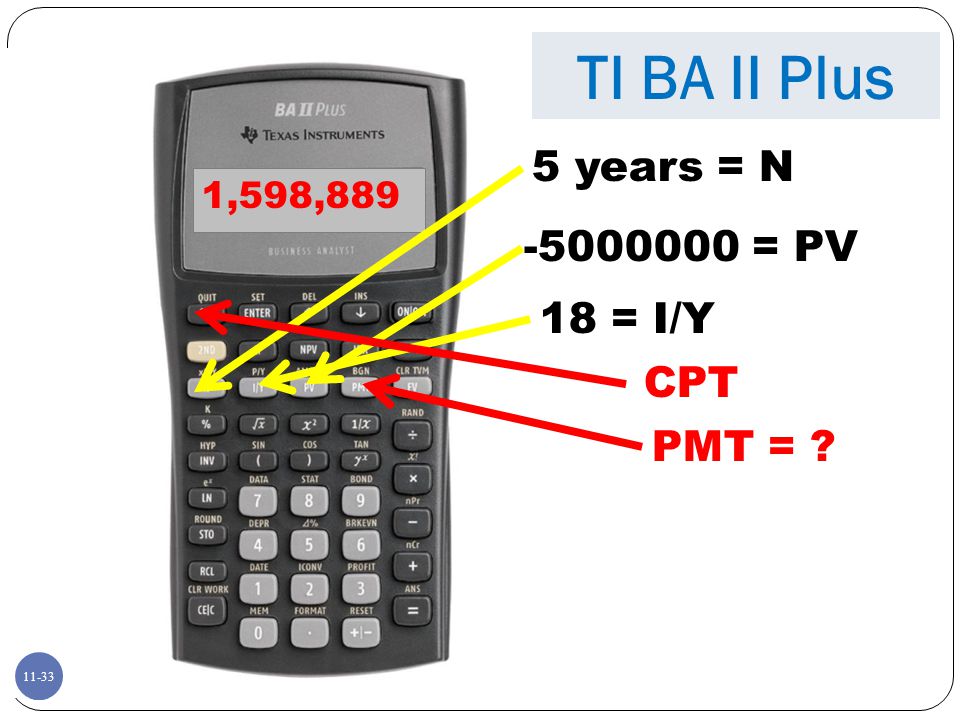
Similar process to that of finding the bid price. You can use your finance calculator to solve this. What OCF (or payment) makes NPV = 0? N = 5; PV = 5,000,000; I/Y = 18; CPT PMT = 1,598,889 = OCF Q = (1,000, ,598,889) / (25,000 – 15,000) = 260 units The question now becomes: Can we sell at least 260 units per year? Assumptions: Cash flows are the same every year, no salvage and no NWC. If there were salvage and NWC, you would net it out to year 0 so that all you have in future years is OCF. Students often are seeking a definitive answer to this problem when in fact, the issue is all about productivity and sales, not really about finance per se. Can the organization sell 260 units is a question left for the sales/marketing personnel.

TI BA II Plus 5 years = N -5000000 = PV 18 = I/Y CPT PMT = ? 1,598,889
11-33

HP 12-C 5 years = N = PV 18 = i PMT = ? 1,598,889

Operating Leverage Leverage in finance is just like that in physics where a small change in one thing produces a large change in another.

Effects of Leverage

Effects of Leverage Small change Large change

Operating Leverage Operating leverage is the relationship between sales and operating cash flow A small change in sales can yield a large change in operating cash flow Operating leverage looks at fixed costs and variable costs. Financial leverage looks at debt and equity. Financial leverage (and combined leverage) are topics in a future chapter.

Degree of Operating Leverage
Degree of operating leverage measures the relationship between sales and operating cash flow The higher the DOL, the greater the variability in operating cash flow The higher the fixed costs, the higher the DOL DOL depends on the sales level you are starting from. DOL = 1 + (FC / OCF)

Example: DOL Consider the previous example Suppose sales are 300 units
This meets all three break-even measures What is the DOL at this sales level? OCF = (25,000 – 15,000)*300 – 1,000,000 = $2,000,000 DOL = 1 + 1,000,000 / 2,000,000 = 1.5

Example: DOL What will happen to OCF if unit sales increases by 20%?
Percentage change in OCF = DOL*Percentage change in Q = 1.5(.2) = .3 or 30% OCF would increase to: 2,000,000(1.3) = $2,600,000 Thus, if unit sales increases by 20%, then the Operating Cash Flow (OCF) would increase by not 20% but 30% demonstrating the effect of operating leverage. A small change in sales yields a much bigger change in OCF.

Capital Rationing Capital rationing occurs when a firm or division has limited resources Soft rationing – the limited resources are temporary, often self-imposed by the corporation. Hard rationing – capital will never be available for this project. If you face hard rationing, you need to reevaluate your analysis. If you truly estimated the required return and expected cash flows appropriately and computed a positive NPV, then capital should be available. Lecture Tip: In 2008, the economy was suffering from a real estate and credit crisis. As a result, lenders essentially withdrew from the market and credit dried up. This is a perfect example of an issue that would create a situation very close to Hard Rationing for many businesses.

Capital Rationing Capital rationing occurs when a firm or division has limited resources The profitability index is a useful tool when a manager is faced with soft rationing to help select the best project for a firm at that time. The Profitability Index is defined and an example is presented in the chapter on capital budgeting techniques.

Ethics Issues Is it ethical for a medical patient to pay for a portion of R&D costs (since experimental procedures are not covered by insurance) prior to the introduction of the final product? Is it proper for physicians to recommend this procedure when they have a vested financial interest in its usage? Case: Researchers associated with South Miami Hospital (SMH) developed a new experimental laser treatment for heart patients. Its development team and the physicians who use the laser consider it to be a lifesaving advance. It should be noted that the physicians who are touting the laser hold a significant stake in the company that produces the laser. To offer a substitute for a balloon angioplasty to treat heart blockages, the experimental laser was developed at a cost of $250,000. SMH estimates that it will cost $20,000 to install the laser. The procedure requires a nurse at $50 per hour, a technician at $30 per hour, and a physician who is paid $750 per hour. Patients are billed $3,000 for the procedure compared to $1,500 for the traditional balloon treatment. Now ask the students to determine the break-even quantity for the new procedure: Fixed cost = 250, ,000 = 270,000 Variable cost = = 830 per hour Cash Break-Even = 250,000 / (3,000 – 830) = hours, or approximately 116 patients (assuming a one-hour procedure per patient).

Quick Quiz What is sensitivity analysis, scenario analysis and simulation? Why are these analyses important, and how should they be used? What are the three types of break-even analysis, and how should each be used? What is the degree of operating leverage? What is the difference between hard rationing and soft rationing?

Comprehensive Problem
A project requires an initial investment of $1,000,000 and is depreciated straight-line to zero salvage over its 10-year life. The project produces items that sell for $1,000 each, with variable costs of $700 per unit. Fixed costs are $350,000 per year. What is the accounting break-even quantity, operating cash flow at accounting break-even, and DOL at that output level? Accounting break-even: Q = (FC + D) / (P – V) = ($350,000 + $100,000) / ($1,000 - $700) = 1,500 units OCF = ( S – VC – FC – D) + D = (1,500 x $1,000 – 1,500 x $700 - $350,000 - $100,000) + $100,000 = $100,000 DOL = 1 + (FC / OCF) = 1 + ($350,000 / 100,000) = 4.5

Terminology Scenario Analysis Sensitivity Analysis Simulation Analysis
Break-even Analysis Operating Leverage Capital Rationing

The degree of operating leverage:
Formulas Accounting Break-Even: NI = (Sales – VC – FC – D)(1 – T) = 0 QP – vQ – FC – D = 0 Q(P – v) = FC + D Q = (FC + D) / (P – v) The degree of operating leverage: DOL = 1 + (FC / OCF)

Key Concepts and Skills
Differentiate between future estimates and certainty Summarize scenario and sensitivity analysis Describe the various forms of break-even analysis Compute operating leverage and explain the components Explain capital rationing and its effects

What are the most important topics of this chapter?
Recognize that future cash flow estimates are uncertain. Scenario, sensitivity, and simulation analyses focus on the risk of uncertainty of cash flows. Break-even analysis looks at the relationship between sales volume and profitability.

What are the most important topics of this chapter?
Operating leverage compares fixed costs and variable costs with respect to operating cash flows. Capital rationing recognizes that economic times often dictate availability of funding for even worthy capital projects.

Questions?

Project Analysis and Evaluation

Similar presentations

Presentation on theme: "Project Analysis and Evaluation"— Presentation transcript:

Similar presentations

About project

Feedback

Log in

Auth with social network:

Project Analysis and Evaluation

Similar presentations

Presentation on theme: "Project Analysis and Evaluation"— Presentation transcript:

Similar presentations

About project

Feedback