2. MaxEnt 2007 Saratoga Springs, NY
Computing the Probability
Of Brain Connectivity with
Diffusion Tensor MRI
JS Shimony
AA Epstein
GL Bretthorst
Neuroradiology Section
NIL and BMRL

3. Part 1: Diffusion Tensor (DT) MRI (Brain Connectivity later)
Diffusion MR images can measure water proton displacements at the cellular level
Probing motion at microscopic scale (mm), orders of magnitude smaller than macroscopic MR resolution (mm)
This has found numerous research and clinical applications
Short introduction

4. Diffusion: Left MCA stroke
Clinical use

5. Standard Spin Echo Mz
Mxy
Mxy
echo 90
180
RF/RO Gz

6. Diffusion Spin Echo
M=Mxyexp(-bD) Mz
Mxy
echo 90
180
RF/RO Gz D

7. Diffusion: Pulse Sequence90
180
Echo Train RF
Gss
EPI Readout
Gro
Multi directional
Gpe

8. Anisotropic Diffusion in WM Fibers
Fibers give anisotropy

9. Diffusion: Single Direction
Example of anisotropy

10. Diffusion Tensor Imaging Model
Basser et al., JMR, 1994 (103) 247
Uses 8 parameters (D ≠ data) λ1 λ2 λ3
The basic model

11. How Diffusion is Measured by MRI
Signal Amplitude
Example of signal decay with gradients
Diffusion Sensitization (q)
Image courtesy: C. Kroenke

12. Image courtesy: C. Kroenke
Diffusion Anisotropy
Signal Amplitude
Example of anisotropy
Diffusion Sensitization (q)
Image courtesy: C. Kroenke

13. Mean Diffusivitiy λ1 λ2 λ3
Key parameters MD
Mean Diffusivity is the average of the diffusion in the different directions

14. Diffusion Anisotropy RA=0 RA<1
Anisotropy is normalized standard deviation of diffusion measurements in different directions
FA and RA most common
Range from 0 to 1
RA=0
Key parameters - anisotropy
RA<1

15. Baseline image / Anisotropy

16. Color Diffusion

17. Part 2: Brain Connectivity
DT data provides a directional tensor field in the brain, used to map neuronal fibers
Detailed WM anatomy used in:
Pre-surgical planning
Neuroscience interest in functional networks
Previously could only be done using cadavers or invasive studies in primates
Termed DT Tractography (DTT)

18. 3D Diffusion Tensor Field

19. Example of Streamline Tracking

20. Streamline DTT Advantages: Disadvantages:
Conceptually and computationally simple
Was the first to be developed
Disadvantages:
Limited to high anisotropy, high signal areas
Can only produce one track
Can’t handle track splitting
Has the greatest difficulty with crossing fibers

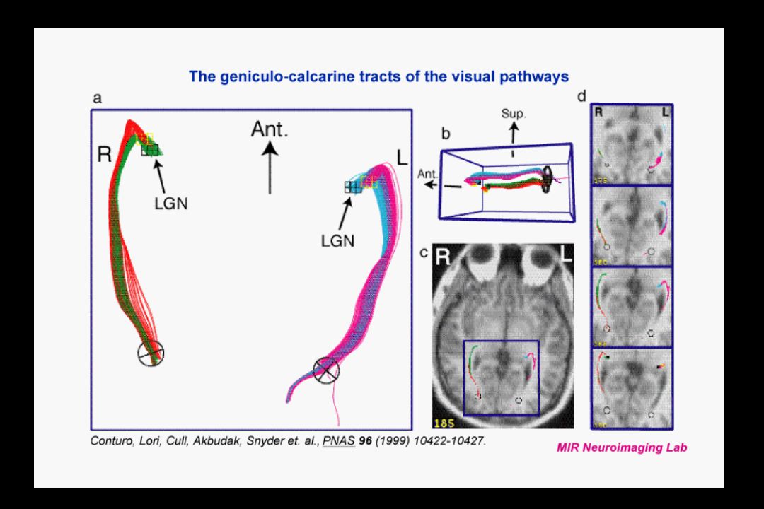
22. Applications: Anatomy
Jellison
AJNR 25:356

23. DTT and Crossing Fibers
Major limitation of current methods of DTT
Difficult to resolve with current methods and SNR
Volume averaging effects
Known areas in the brain
Decrease sensitivity and specificity, distorts connection probabilities

24. Crossing Fibers Locations

25. Probabilistic DTT Behrens et al. MRM 2003 50:1077-1088 Advantages:
Better accounts for experimental errors
More robust tracking results
Better deals with crossing fibers, low SNR
Disadvantages:
Computationally intense
Probabilities will be modified by crossing fibers

26. Probabilistic Tractography
Express DT parameters for pixel i
Since each pixel is independent in this model the probability for the DT parameters given the data D can be factored:

27. Utilize Angular Error Estimations
pdf
Cone of angular
uncertainty
Low Anisotropy High Anisotropy

28. Probabilistic Tracking
End
zone
Start
zone

29. Example Probabilistic DTT

30. Part 3: Methods and Results
Use prior information!!!
Assumption of pixel independence is non_biological
Nerve fiber bundles can travel over long distances in the brain and cross many pixels
Incorporate this into the model via a:
“Nearest Neighbor Connectivity Parameter”

31. Adding the Connectivity Parameter
Add nearest neighbor connectivity parameter
No independence between the pixels
Each pixel depends on its neighbors via the prior of its connectivity

32. Connectivity Parameter Prior

33. Adding Connectivity Parameter
The preference for connectivity is indicated by the prior for Lij
Express this as the probability that a water molecule will diffuse from pixel i to j

34. Parallel Processing Details
Connection between neighboring pixels complicates the calculations
When processing on a parallel computer, the values of the neighbors cannot change
Example in 1D and 2D

35. Method: 3x3x3 Simulation

36. Results: Connectivity Parameter

37. Coronal Section in Crossing Fiber area

38. Anatomy Comparison

39. Results: Connectivity Parameter

40. Summary
DT imaging provides accurate estimation of the tensor field of the WM in the brain
Accurate estimation of the connectivity between different brain regions is of great clinical and research interest
Prior work has assumed independent pixels
Prior information on local connectivity may provide a more accurate representation of the underlying tissue structure
Acknowledgements: NIH K23 HD053212, NMSS PP1262, and Chris Kroenke