Quantitative Hydrology

Quantitative Hydrology
Basin Recharge and Runoff As rain fall towards the earth, a portion of it is intercepted by the leafs and stems of vegetation. The water so retained, interception, together with depression storage and soil moisture, constitutes basin recharge.

Interception Interception is that portion of precipitation which, while falling, is intercepted by aerial portion of vegetation, buildings and other objects above the surface of earth and evaporates back to the atmosphere. The adhesive force between the water drops and the vegetation holds back the drops of water against gravity until they grow in size to over weigh and slip down.

Interception Factors on which interception depends are:
(a) Intensity and duration of the storm, (b) Density of trees, (c) Type of trees (i.e. long or short, coniferous or deciduous, area of canopy) and other obstructions, (d) Season of the year and (e) Wind velocity at the time of precipitation.

IL = aP + b (1 – e (-p / b)) where
Interception The part of precipitation retained by the aerial portion of vegetation and other objects and is either absorbed by them or evaporates back is called interception loss. Depending on the vegetal cover and precipitation, a general form of equation for interception loss can be written as: IL = aP + b (1 – e (-p / b)) where

Interception a and b are constants which depend on the factors of infiltration loss, a varies between 0.01 and 0.2 and b between 2.5 and 38% of rainfall P is the precipitation depth in mm.

Interception Example: Calculate the interception loss for a tropical forest area in India (a = 0.11 and b = 15% of P). The intensity of precipitation is low but uniform over the area. Total depth of storm rainfall is 4 cm.

Interception Solution: Here a = 0.11, b = 0.15P, P = 4.0 cm
Interception loss IL = aP + b (1 – e (-p / b)) IL = 0.11P P (1 – e (-p/0.15P)) = P = cm = 10.4 mm.

Depression Storage Any natural ground surface generally has numerous shallow depressions of varying size, shape and depth. When precipitation fall, these depressions form miniature reservoirs detaining water temporarily. Water from these storages either evaporates or infiltrates into the ground charging the ground water reservoir.

Depression Storage After filling all the small depressions, overland flow from the area takes place. Due to change in land use pattern, depression storages also change with time, which makes it almost a non-measurable quantity.

Depression Storage The important factors affecting depression storage are: (a) land form, (b) soil characteristics, (c) topography, (d) antecedent precipitation index and (e) man made disturbances, like terrace farming.

Depression Storage Depression storage helps to reduce soil erosion and increase soil moisture content. Therefore, farmers are encouraged to go for terrace farming to conserve soil and rain water for beneficial uses. The sum of infiltration and depression storage can vary from 10 to 50 mm per storm depending on their intensity, duration and other characteristics.

Infiltration and Its Estimation
Infiltration is as the entry or the passage of water into the soil through soil surface. It is a major loss of precipitation affecting runoff of a basin.

This term should be properly understood and quantified. Losses like interception, depression storage and evaporation during precipitation are small, which cannot change the runoff of a basin significantly during major floods, but infiltration is a major process continuously affecting the magnitude, timing and distribution of surface runoff at any measured outlet of a basin. It is responsible for the growth and nourishment of life on earth.

Infiltration process is initiated by creation of hydrogen bond between soil particles and the water. The adhesive force of attraction between soil and water, the surface tension, capillarity and gravitational forces help to force more water between the pores of soil particles as more water is added to the system due to rain.

Infiltration capacity is the maximum rate at which a given soil can absorb water under a given set of conditions at a given time. At any instant the actual infiltration, can be equal to infiltration capacity only when the rainfall intensity is greater than infiltration capacity, otherwise actual infiltration will be equal to the rate of rainfall. This can be observed during low intensity rainfall when there is no surface runoff produced due to precipitation.

Once water enters into the soil, the process of transmission of water within the soil known as percolation takes place, thus removing the water from near the surface to down below, charging the ground water reservoir.

Infiltration and percolation are directly interrelated. When percolation stops, infiltration also stops. During any storm, infiltration is the maximum at the beginning of the storm, decays exponentially and attains a constant value as the storm progresses.

The effect of infiltration is to: reduce flood magnitude delay the time of arrival of water to the channel reduce the soil erosion recharge to the ground water reservoir fill the soil pores with water to its field-capacity, which subsequently supply water to the plants avail the ground water during the non-rain periods in the channels help to supply water to plants

Factors Affecting Infiltration
Factors affecting infiltration depend on both meteorological and soil medium characteristics. These are: Surface Entry: If a soil surface is bare, the impact of raindrops causes in-washing of finer particles and clogs the surface. This retards infiltration. An area covered by grass and other bushy plants has better infiltration capacity than a barren land.

Percolation: For infiltration to continue, water that has entered the soil must be transmitted down by the force of gravity and capillary actions. When percolation rate is slow, the infiltration rate is bounded by the rate of percolation. This depends on the factors like type of soil, its composition, permeability, porosity, stratification, presence of organic matter and presence of salts.

Antecedent Moisture Condition: Infiltration depends on the presence of moisture in the soil. For the second storm in succession, the soil will have lesser rate of infiltration than the first maiden storm of the season. Except sandy soil most other soils have swelling ingredients, which swells in presence of water and reduce infiltration rate to the extent of their presence

Rainfall Intensity and Duration: During heavy rainfall, the top soil is affected by mechanical compaction and by the in-wash of finer materials. This leads to faster decrease in the rate of infiltration than with low intensities of rainfall. Duration of rain affects to the extent that when the same quantity of rain falls in n number of isolated storms instead of a continuous one, the infiltration will be higher in the former case

Human Activities: When crops are grown or grass covers a barren land, the rate of infiltration is increased. On the other hand construction of roads, houses, overgrazing of pastures and playgrounds reduce infiltration capacity of an area considerably

Depletion of Ground Water Table: Position of ground water table should not be very close to the surface for infiltration to continue. The quantity of infiltrated water entering into the soil should be drained out fully from the top soil zone so that there is some space available for infiltrated water to store during the next rain

Quality of Water: Water containing silt, salts and other impurities affect the infiltration to the extent they are present. Salts present affect the viscosity of water and may also react chemically with soil to form complexes which obstruct the porosity of soil, thereby affecting infiltration. Silts clog the pore spaces retarding infiltration rate considerably

Field Measurement Using Infiltrometers
Two types of infiltrometers used are: Single cylindrical and Concentric double cylindrical.

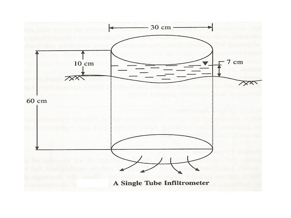
Single Tube lnfiltrometer
It consists of a hallow metal cylinder 30 cm in diameter and 60 cm long driven into the ground such that 10 cm of it projects above ground level. Water is poured at the top such that a head of 7 cm within the infiltrometer is maintained above ground level. A graduated jar or burette is used to add water, to give directly the volume of water added over time.

Single Tube lnfiltrometer
A plot of time in abscissa against rate of water added in mm/h gives an infiltration capacity curve for the area. The setup resembles to the flooding type of irrigation situation in the field which can be a possible representation of real local conditions. Sufficient precautions should be taken to drive the cylinder into the ground with minimum disturbance to the soil structure. In a single infiltrometer, the major criticism is that water spreads out immediately beyond the bottom of the cylinder which does not represent a true infiltration condition of the field

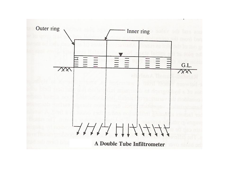
Double Tube lnfiltrometer
To overcome the objections of a single ring infiltrometer a set two concentric hollow cylinders of same length are used. Water is added to both the rings to maintain the same height. Reading of the burette for the inner cylinder is taken as infiltration capacity of the soil. The outer cylinder is maintained to prevent spreading of water from the inner one.

Double Tube lnfiltrometer
The important disadvantages still prevalent in these types of infiltrometers are: The size effect: Larger diameter infiltrometers give more accurate and always lesser value of infiltration than smaller diameter type. Boundary effect. Disturbance of original soil due to driving of the rings.

Field Measurement Using Infiltrometers
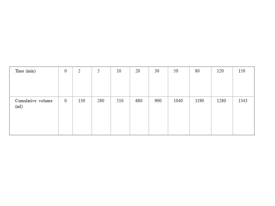
Example: From a double tube infiltrometer with inside ring diameter of 30 cm, the following observations were taken. Plot the infiltrations capacity curve and find the constant rate of infiltration that the experimental field have towards the end.

Time (min) 2 5 10 20 30 50 80 120 150 Cumulative volume (ml) 130 280 510 680 900 1040 1190 1280 1343

Solution Area of the infiltrometer = (/4) 302 = cm2

Rainfall-Runoff Analysis
A network of rain gauges gives the average storm precipitation over a basin. The runoff from the basin can be measured at the outlet or at the desired location by gauging the stream. The difference between precipitation and the corresponding runoff averaged over the basin over time should give the total loss. This should form the basis for the estimation of infiltration.

During storms, evapotranspiration is negligible. Depression storage and interception can be estimated as discussed earlier. The balance gives a true representation of the basin infiltration losses..

The infiltration capacity of a soil at any time is the maximum rate at which water will enter the soil. The infiltration rate is the rate at which water actually enters the soil during a storm; and it must equal the infiltration capacity or the rainfall rate, whichever is less. An ideal infiltration capacity curve proposed by Horton (1933) is ft = fc + (fo - fc) e-kt

where ft = the infiltration capacity at any time t from the beginning of the storm in mm/h. fc = the infiltration rate in mm/h at the final steady stage when the soil profile becomes fully saturated fo = the maximum initial value when t = 0 in mm/h at the beginning of the storm k = empirical constant depending on soil cover complex, vegetation and other factors t = time lapse from the onset of the storm

A typical curve of ft separating the rainfall intensity histogram between infiltration and surface runoff is

Since we are interested in determining the infiltration rate for storms of large basins, an average infiltration rate known as infiltration index is assumed. This type of assumption underestimates infiltration rate during the initial part of the storm and slightly overestimates towards the end of it.

The assumption holds fairly good for analysis of high intensity and long duration storms or in a situation, when the area is fairly saturated before the onset of the storm. Difficulties with the theoretical approach to infiltration and practical difficulties to determine the values of fo and k, led to the use of infiltration indices based on an empirical approach.

Infiltration Indices The following indices are mostly used for computation of infiltration rate from rainfall runoff data: -Index W-Index

Infiltration Indices/ -Index
The average rate of rainfall above which the rainfall volume equals to runoff volume is called -Index.  = I – R in which R = a I1.2 I = the rainfall intensity in mm/h on a daily (24 h) basis R = the runoff in mm.

For computation of R, take I in mm/day and for computation of , divide R by 24 to convert it to mm/h. Values of coefficient a vary from 0.17 to For sandy soils it may be taken as 0.20, coastal alluvium 0.25 to 0.30, silt 0.35, red and clayey soil 0.40, black cotton soil 0.45 and hilly soil 0.50.

Infiltration Indices/ W-Index
This index is considered as an improvement over -index in the sense that surface storage and interception losses are considered in its computation. It is defined as the average rate of infiltration which equals to the rate of precipitation minus surface runoff and retention during time t and is expressed as: W = (P - SRo - DR) / t

where P = the total depth of storm rainfall in mm SRo = the total depth of surface runoff in mm DR = the total depth of surface retention (depth of depression storage plus interception loss) mm and t = the time in hour during which rainfall rate exceeds infiltration rate. Obviously when DR = 0, W-index and -index become the same.

Example: the following are the rates of rainfall for successive 20 minutes period of a 140 minutes storm: 2.5, 2.5, 10.0, 7.5, 1.25, 1.25, 5.0 cm/hr. taking the value of -index as 3.2 cm/hr, find out the runoff in cm, the total rainfall, and the value of W-index.

Runoff = (10-3. 2)20/60 + (7. 5-3. 2)20/60 + (5-3. 2)20/60 = (6. 8+4
Runoff = (10-3.2)20/60 + ( )20/60 + (5-3.2)20/60 = ( )20/60 = 4.3 cm Total precipitation = (2.5*20/60) + (2.5*20/60) + (10*20/60) + (7.2*20/60) + (1.25*20/60) + (1.25*20/60) + (5*20/60) = ( )20/60 = 10 cm W-index = (P - SRo - DR) / t (10-4.3)140/60 = 2.44 cm/hr

Hydrograph Analysis The characteristics of direct and groundwater runoff differ so greatly that they must be treated separately in problems involving short-period, or storm, runoff. There is no practical means of differentiating between groundwater flow and direct runoff after they have been intermixed in the stream, and the techniques of hydrograph analysis are arbitrary.

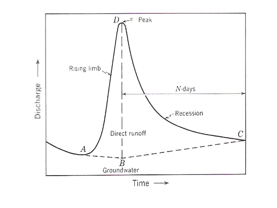
Hydrograph Analysis The typical hydro graph resulting from a single storm consists of a rising limb, peak, and recession. The recession represents the withdrawal of water stored in the stream channel during the period of rise. Double peaks are sometimes caused by the geography of the basin but more often result from two or more periods of rainfall separated by a period of little or no rain.

Hydrograph Analysis Numerous methods of hydrograph separation have been used. The method illustrated by ABC in Figure is simple and as easily justified as any other. The recession of flow existing prior to the storm is extended to point B under the crest of the hydrograph. The straight line BC is then drawn to intersect the recession limb of the hydrograph N days after the peak.

Hydrograph Analysis The value of N is not critical and may be selected arbitrarily by inspection of several hydrographs from the catchment. The selected value should, however, be used for all storm events analyzed to conform to the unit hydrograph concept. The time N will increase with size of drainage basin since a longer time is required for water to drain from a large basin than from a small one. A rough guide to the selection of N (in days) is N = Ad0.2 Where Ad is the drainage area in square miles. With Ad in square kilometers, computed values of N should be reduced by about 20 percent.

Unit Hydrographs If two identical rainstorms could occur over a catchment with identical conditions prior to the rain, the hydrographs of runoff from the two storms would be expected to be the same. This is the basis of the unit hydrograph concept.

Unit Hydrographs Actually the occurrence of identical storms is very rare. Storms may vary in duration, amount, and aerial distribution of rainfall. A unit hydrograph is a hydrograph with a volume of 1 in. (25 mm) of direct runoff resulting from a rainstorm of specified duration and aerial pattern. Hydrographs from other storms of like duration and pattern are assumed to have the same time base, but with ordinates of direct runoff in proportion to the runoff volumes.

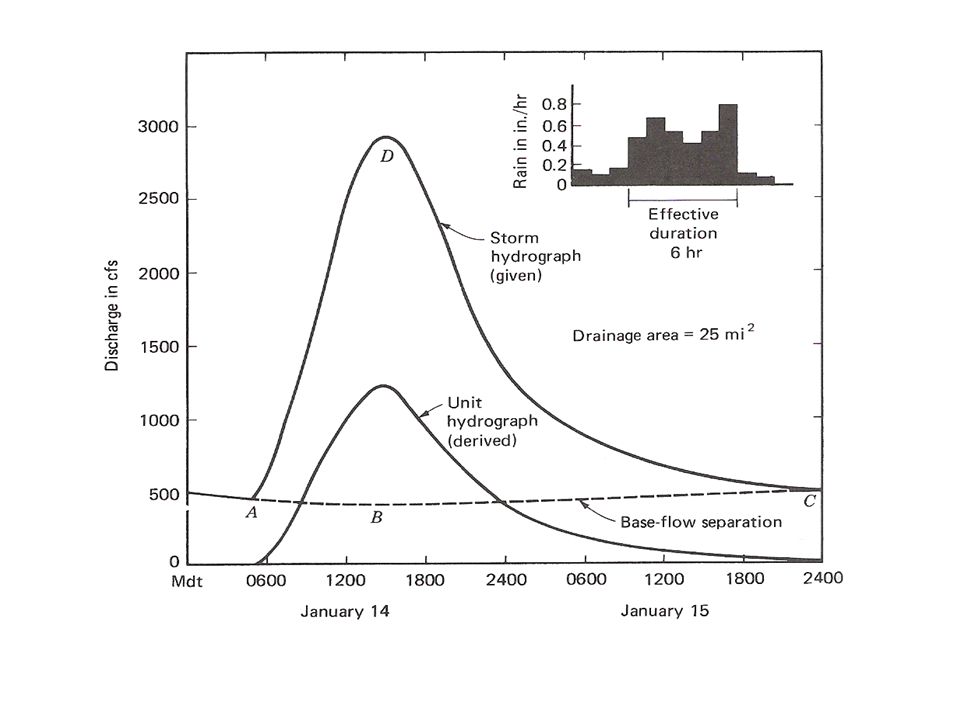
Unit Hydrographs A unit hydrograph may be constructed from the rainfall and stream flow data of a storm with reasonably uniform rainfall intensity and without complications from preceding or subsequent rainfall. The first step in the derivation is the separation of groundwater flow from direct runoff. The volume of direct runoff (area ABCD, Figure) is determined and the ordinates of the unit hydrograph are found by dividing the ordinates of the direct runoff by the volume of direct runoff in inches (or cm). The resulting unit hydrograph should represent a unit volume (1 in.) of runoff, or 1 cm in metric units.

Unit Hydrographs Example: Derive a unit hydrograph from the flows indicated by the previous Figure. Solution: Since a unit hydro graph applies to direct runoff, the first step is the estimation of this quantity. The groundwater hydrograph (i.e., base flow) is assumed to follow the recession occurring before the storm to a point under the peak of the total hydrograph (point A to point B). From B the base flow is assumed to increase slowly to point C. In this case the location of point C was chosen arbitrarily.

Unit Hydrographs The table that follows illustrates the other steps in the process. After entering the date and time, the total flow is tabulated in the third column and the corresponding base flow is entered in column 4. Subtracting base flow from total flow gives the direct runoff values (column 5). Summing the direct runoff ordinates gives the total direct runoff, which must be converted to inches of depth over the 25-mi2 catchment: 11,970 x (3/24) = 1496 cfs-days

Unit Hydrographs In this calculation it is assumed that each entry in the table represents an average flow for 3 hr, that is, 3/24 day. Summing these flows and multiplying by 3/24 gives the volume of runoff for the storm in cfs-days. There are 26.9 cfs-days in 1 in. of runoff from 1 mi2. Hence the volume of direct runoff in inches over the 25-mi2 catchment is: 1496/(25 x 26.9) = 2.22 in.

Unit Hydrographs Dividing each ordinate of direct runoff by 2.22 gives the ordinates of the unit hydrograph (column 6). The final step is the assignment of an effective storm duration from a study of the rainfall records.

Date Hour Total flow (given) Base Direct runoff Ordinates of unit hydrograph (derived) Hours after start (1) (2) (3) (4) (5) (6) (7) 14 0500 470 0800 1200 440 760 342 3 1100 2250 410 1840 829 6 1400 2920 380 2540 1145 9 1700 2670 400 2270 1022 12 2000 2060 1650 743 15 2300 1430 420 1010 455 18 0200 430 670 302 21 910 212 24 780 450 330 149 27 680 460 220 99 30 600 130 59 33 540 480 60 36 510 490 20 39 500 42 11 ,970

Unit Hydrographs Data from at least one recording rain gage is necessary. Periods of low-intensity rain at the beginning and end of the storm should be ignored if they did not contribute substantially to the total runoff. In this case the effective storm duration is 6 hr, and the unit hydrograph is called a 6 hr unit hydrograph. The use of a unit hydrograph to estimate the hydrograph of a storm of like duration is illustrated in the following example.

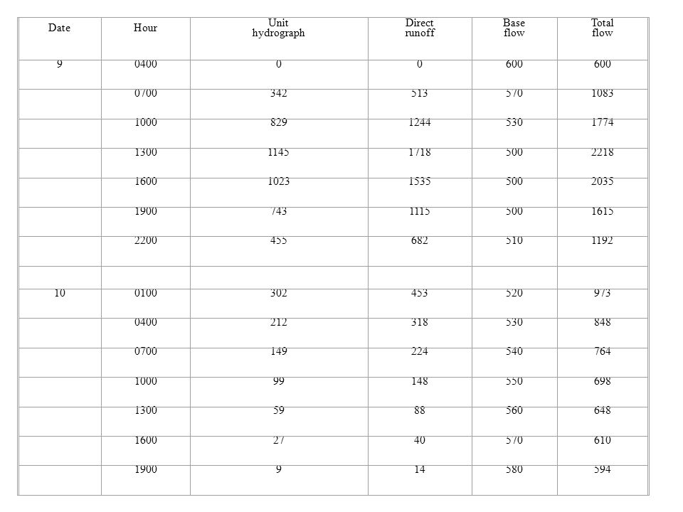
Unit Hydrographs Example: A storm occurs between 0400 and 1000 hours. The estimated depth of direct runoff is 1.5 in. Construct the hydrograph to be expected from this storm. Solution: Assume the initial flow in the stream is 600 cfs. All flows in the table that follows are in cubic feet per second. .

Date Hour Unit hydrograph Direct runoff Base flow Total 9 0400 600 0700 342 513 570 1083 1000 829 1244 530 1774 1300 1145 1718 500 2218 1600 1023 1535 2035 1900 743 1115 1615 2200 455 682 510 1192 10 0100 302 453 520 973 212 318 848 149 224 540 764 99 148 550 698 59 88 560 648 27 40 610 14 580 594

Unit Hydrographs The flow occurring prior to the storm serves as a starting point for the line ABC representing the base flow or estimated groundwater flow. In this example it has been assumed to decrease slowly to the time of peak and then to rise slowly to meet the estimated direct runoff 33 hr after the peak. The ordinates of the unit hydrograph are taken from previous example and multiplied by the estimated depth of direct runoff to generate the hydrograph of direct runoff. The direct runoff is added to the ground water flow to obtain the total hydrograph (ADC). The direct runoff was estimated by one of the methods discussed earlier in this course.

Unit Hydrographs The number of unit hydrographs for a given catchment is theoretically infinite since there could be one for every possible duration of rainfall and every possible distribution pattern. Practically there need be only a few relatively short durations considered, since these short durations can be used to build a hydrograph for a longer duration .

Unit Hydrographs The effect of varying aerial patterns of rainfall can be minimized by restricting the use of unit hydrographs to relatively small catchments. An area of 2000 mi2 (5000 km2) is often taken as an upper limit. The effect of exceeding this limit will decrease the accuracy of computed hydrographs. Where rainfall is typically in the form of showers or thunderstorms covering small areas, the unit hydrograph is applicable only to very small catchments.

Unit Hydrographs Hydrographs for larger catchments can be estimated by dividing the area into sub-catchments and summing the flows from these sub-catchments using routing techniques. The application of a 3-hr unit hydrograph to a storm of 12 hr duration 6 illustrated in the following example.

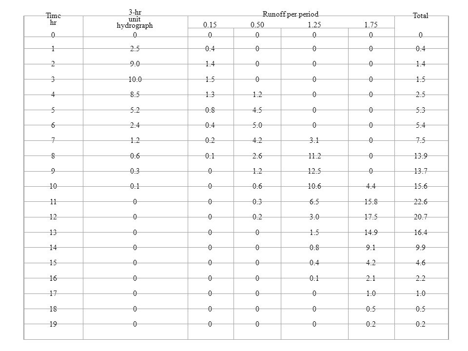
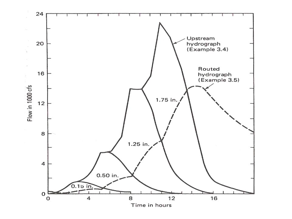
Unit Hydrographs Example: Develop the hydrograph of direct runoff from a 12-hr storm on a given catchment whose 3-hr unit hydrograph is given in the first two columns of the following table. The 12-hr storm occurs in four 3-hr periods having estimated runoffs of 0.15, 0.50, 1.25, and 1.75 in. Solution: The computations are illustrated in the following table. Base flow is ignored. Flows are in 1000 cfs.

Time hr 3-hr unit hydrograph Runoff per period Total 0.15 0.50 1.25 1.75 1 2.5 0.4 2 9.0 1.4 3 10.0 1.5 4 8.5 1.3 1.2 5 5.2 0.8 4.5 5.3 6 2.4 5.0 5.4 7 0.2 4.2 3.1 7.5 8 0.6 0.1 2.6 11.2 13.9 9 0.3 12.5 13.7 10 10.6 4.4 15.6 11 6.5 15.8 22.6 12 3.0 17.5 20.7 13 14.9 16.4 14 9.1 9.9 15 4.6 16 2.1 2.2 17 1.0 18 0.5 19

Unit Hydrographs The 3-hr unit hydro graph was developed through analysis of several 3-hr storms using the procedure illustrated in the previous example. The depth of direct runoff for each 3-hr period of the storm is estimated by subtracting an estimate of the infiltration from the rainfall during the period. The unit hydrograph ordinates are multiplied by 0.15, 0.50, 1.25, and 1.75, respectively, each lagged by 3 hr from the previous increment. The resulting values are summed to give the total hydrograph of composite storm.

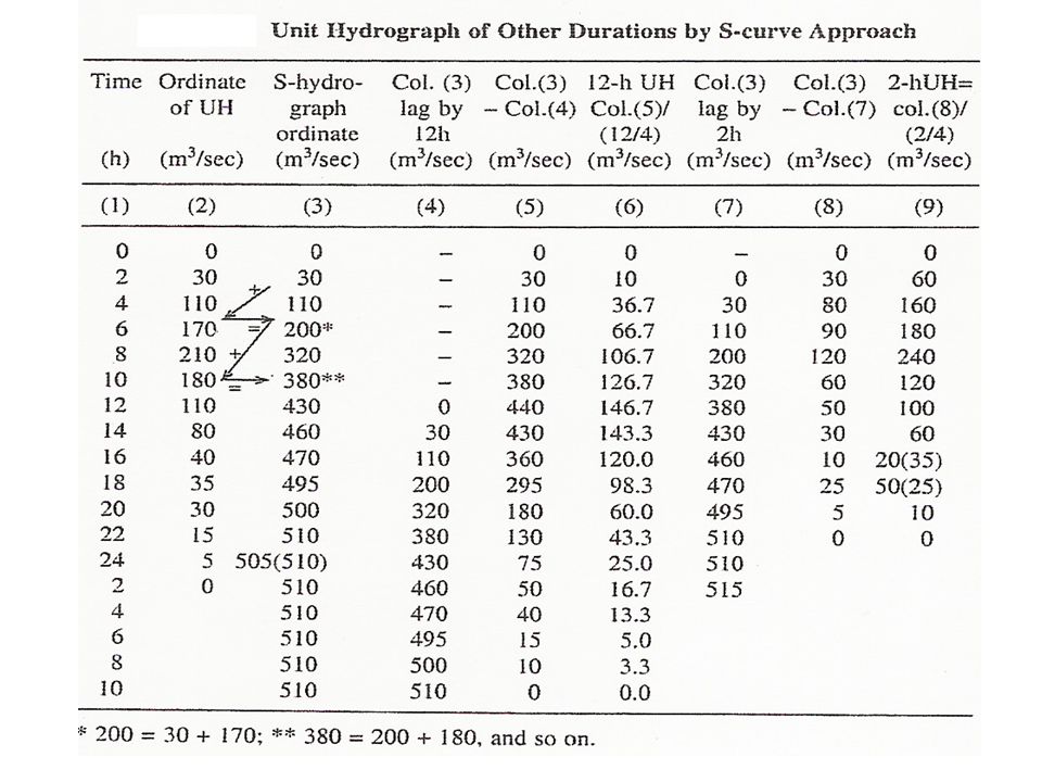
Example: A 4 h hydrograph for a Basin is given below
Example: A 4 h hydrograph for a Basin is given below. Calculate (i) A 12-h unit hydrograph and (ii) 2-h UH by S-hydrograph approach. Solution: Required S- hydrograph from the given 4-h.UH is calculated in the following table.

Synthetic Unit Hydrograph
The unit hydrograph from rainfall and stream flow data on a watershed applies only for that watershed and for the point on the stream where the stream flow data were measured. Synthetic unit hydro graph procedures are used to develop unit hydrographs for other locations on the stream in the same watershed or for nearby watersheds of a similar character.

Synthetic Unit Hydrograph
There are three types of synthetic unit hydrographs: (1) Those relating hydro graph characteristics (peak flow rate, base time, etc.) to watershed characteristics (Snyder, 1938; Gray, 1961), (2) Those based on a dimensionless unit hydrograph (Soil Conservation Service, 1972), and (3) Those based on models of watershed storage (Clark, 1943).

Snyder's Synthetic Unit Hydrograph
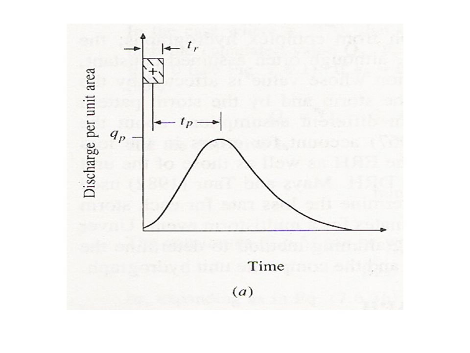
In a study of watersheds located mainly in the Appalachian highlands of the United States, and varying in size from about 10 to 10,000 mi2 (30 to 30,000 km2), Snyder (1938) found synthetic relations for some characteristics of a standard unit hydro graph [Figure below].

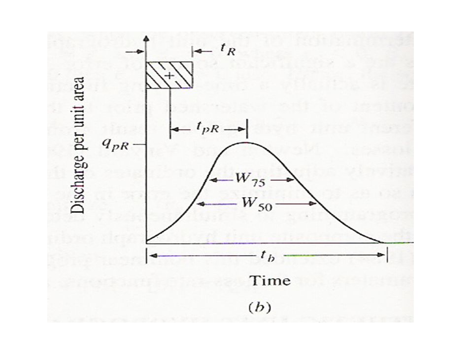
From the relations, five characteristics of a required unit hydro graph [Figure below] for a given excess rainfall duration may be calculated: the peak discharge per unit of watershed area, qpR, the basin lag tpR (time difference between the centroid of the excess rainfall hyetograph and the unit hydro graph peak), the base time tb, and the widths W (in time units) of the unit hydro graph at 50 and 75 percent of the peak discharge.

Using these characteristics the required unit hydro graph may be drawn
Using these characteristics the required unit hydro graph may be drawn. The variables are illustrated in Figure below.

Snyder defined a standard unit hydrograph as one whose rainfall duration tr, is related to the basin lag tp by tp = 5.5 tr For a standard unit hydrograph he found that: 1. The basin lag is tp = C1Ct (L Lc )0.3

where tp is in hours, L is the length of the main stream in kilometers (or miles) from the outlet to the upstream divide, Lc is the distance in kilometers (miles) from the outlet to a point on the stream nearest the centroid of the watershed area, Cl = 0.75 (1.0 for the English system), and Ct is a coefficient derived from gauged watersheds in the same region.

2. The peak discharge per unit drainage area in m 3/s'km2 (cfs/mi 2) of the standard unit hydrograph is qp = C2Cp / tp where C2 = 2.75 (640 for the English system) and Cp is a coefficient derived from gauged watersheds in the same region.

To compute Ct and Cp for a gauged watershed, the values of L and Lc are measured from the basin map. From a derived unit hydrograph of the watershed are obtained values of its effective duration tR in hours, its basin lag tpR in hours, and its peak discharge per unit drainage area, qpR, in m3/s.km2.cm (cfs/mi2.in for the English system). If tpR = 5.5tR, then tR = tr, tpR = tp, and qpR = qp, and Ct and Cp are computed by equations mentioned earlier.

If tpR is quite different from 5.5tR, the standard basin lag is tp = tpR + (tr – tR) / 4 3. The relationship between qp and the peak discharge per unit drainage area qpR of the required unit hydrograph is qpR = (qp tp) / tpR

4. The base time tb in hours of the unit hydrograph can be determined using the fact that the area under the unit hydrograph is equivalent to a direct runoff of I cm (1 inch in the English system). Assuming a triangular shape for the unit hydrograph, the base time may be estimated by tb = C3 / qpR where C3 = 5.56 (1290 for the English system).

5. The width in hours of a unit hydrograph at a discharge equal to a certain percent of the peak discharge qpR is given by W = Cw qpR-1.08 where Cw = 1.22 (440 for English system) for the 75-percent width and 2.14 (770, English system) for the 50-percent width. Usually one-third of this width is distributed before the unit hydrograph peak time and two-thirds after the peak.

Example: From the basin map of a given watershed, the following quantities are measured: L = 150 km, Lc = 75 km, and drainage area = 3500 km2. From the unit hydrograph derived for the watershed, the following are determined: tR = 12 h, tpR = 34 h, and peak discharge = m3/s.cm. Determine the coefficients Ct and Cp for the synthetic unit hydrograph of the watershed.

Solution: From the given data, 5.5tR = 66 h, which is quite different from tpR (34 h). tp=tpR + (tr – tR) / 4 =34 +( tr-12) / 4 tr = 5.9 h and tp = 32.5 h tp = C1 Ct(L Lc)0.3 32.5=0.75Ct(150 x 75)0.3 Ct=2.65

The peak discharge per unit area is qpR = 157.5/3500 = m3/s.km2.cm. The coefficient Cp is calculated with qp,qpR, and tp = tpR: qpR = (C2Cp) / tpR 0.045 = 2.75Cp / 34.0 Cp=0.56

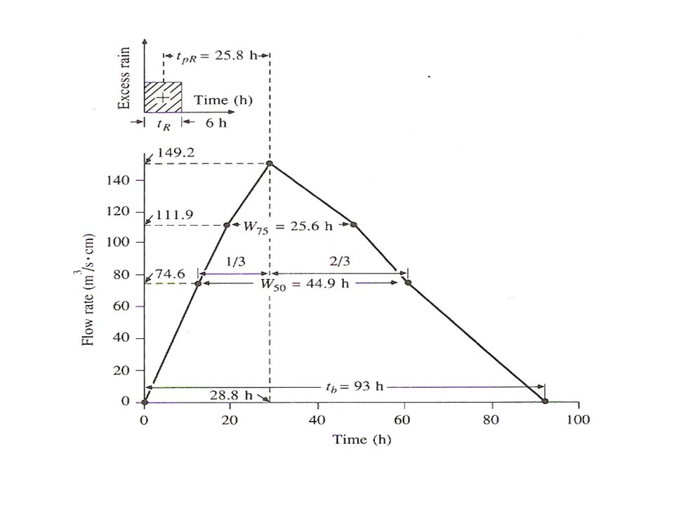
Example: Compute the six-hour synthetic unit hydrograph of a watershed having a drainage area of 2500 km2 with L = 100 km and Lc = 50 km. This watershed is a sub-drainage area of the watershed in previous example.

Solution: The values Ct = 2.64 and Cp = 0.56 determined in previous example can also be used for this watershed. Thus, tp = 0.75 x 2.64 x (100 x 50)0.3 = 25.5 h tr = 25.5/5.5 = 4.64 h

For a six-hour unit hydrograph, tR = 6 h, tpR = tp - (tr - tR) / 4 = 25.5 (4.64-6)/4 = 25.8 h. qp = 2.75 x 0.56/25.5 = m3/s.km2.cm qpR = x 25.5/25.8 = m3/s.km2.cm the peak discharge is x 2500 = m3/s.cm.

The widths of the unit hydrograph are: At 75 percent of peak discharge, W = 1.22qpR-1.08 = 1.22 X l.08 = 25.6 h. A similar computation gives a W = 44.9 h at 50 percent of peak. The base time tb = 5.56/qpR = 5.56/ = 93h. The hydrograph is drawn, as in Figure below and checked to ensure that it represents a depth of direct runoff of 1 cm.

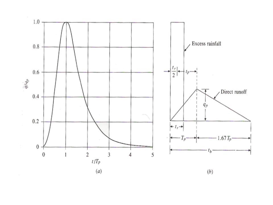
SCS Dimensionless Hydrograph
The SCS dimensionless hydrograph is a synthetic unit hydrograph in which the discharge is expressed by the ratio of discharge q to peak discharge qp and the time by the ratio of time t to the time of rise of the unit hydro graph, Tp.

Given the peak discharge and lag time for the duration of excess rainfall, the unit hydrograph can be estimated from the synthetic dimensionless hydrograph for the given basin. Figure below shows such a dimensionless hydrograph, prepared from the unit hydrographs of a variety of watersheds. The values of qp and Tp may be estimated using a simplified model of a triangular unit hydrograph as shown in Figure below, where the time is in hours and the discharge in m3/s.cm (or cfs/in) (Soil Conservation Service, 1972).

From a review of a large number of unit hydrographs, the Soil Conservation Service suggests the time of recession may be approximated as 1.67 Tp. As the area under the unit hydrograph should be equal to a direct runoff of 1 cm (or 1 in), it can be shown that qp = CA / Tp where C = 2.08 (483.4 in the English system) and A is the drainage area in square kilometers (square miles).

Further, a study of unit hydrographs of many large and small rural watersheds indicates that the basin lag tp  0.6Tc, where Tc is the time of concentration of the watershed. As shown in previous Figure, time of rise Tp can be expressed in terms of lag time tp and the duration of effective rainfall tr Tp = (tr/2) + tp

Example: Construct a 10-minute SCS unit hydrograph for a basin of area 3.0 km2 and time of concentration 1.25 h. Solution: The duration tr = 10 min =0.166 h, lag time tp = 0.6Tc = 0.6 X1.25 = 0.75 h, and rise time Tp = (tr / 2) + tp = (0.166/2) = h. qp = CA / Tp = 2.08 x 3.0/0.833 = 7.49 m3/s.cm.

The dimensionless hydrograph in the previous figure may be converted to the required dimensions by multiplying the values on the horizontal axis by Tp and those on the vertical axis by qp . Alternatively, the triangular unit hydrograph can be drawn with tp = 2.67 Tp = 2.22 h. The depth of direct runoff is checked to equal 1 cm.

Quantitative Hydrology

Similar presentations

Presentation on theme: "Quantitative Hydrology"— Presentation transcript:

Similar presentations

About project

Feedback

Log in

Auth with social network:

Quantitative Hydrology

Similar presentations

Presentation on theme: "Quantitative Hydrology"— Presentation transcript:

Similar presentations

About project

Feedback